Example with CMIP6 models (100 - 500 km)

Table of Contents

• 1. Introduction
• 2. Data Wrangling
• 3. Exploratory Data Analysis
• 4. Conclusion
• 5. References

1. Introduction

Cloud feedbacks are a major contributor to the spread of climate sensitivity in global climate models (GCMs) Zelinka et al. (2020). Among the most poorly understood cloud feedbacks is the one associated with the cloud phase, which is expected to be modified with climate change Bjordal et al. (2020). Cloud phase bias, in addition, has significant implications for the simulation of radiative properties and glacier and ice sheet mass balances in climate models.

In this context, this work aims to expand our knowledge on how the representation of the cloud phase affects snow formation in GCMs. Better understanding this aspect is necessary to develop climate models further and improve future climate predictions.

• Retrieve CMIP6 data through ESGF

• Hybrid sigma-pressure coordinates to isobaric pressure levels of the European Centre for Medium-Range Weather Forecast Re-Analysis 5 (ERA5) with GeoCAT-comb

• Regridd the CMIP6 variables to the exact horizontal resolution with xesmf

• Calculate an ensemble mean of all used models

• Calculate and plot the seasonal mean of the ensemble mean

Questions

• How is the cloud phase and snowfall varying between 2007 and 2010?

NOTE: We answer questions related to the comparison of CMIP models to ERA5 in another Jupyter Notebook.

2. Data Wrangling

This study will compare surface snowfall, ice, and liquid water content from the Coupled Model Intercomparison Project Phase 6 (CMIP6) climate models to the European Centre for Medium-Range Weather Forecast Re-Analysis 5 (ERA5) data from 2006 to 2009. We conduct statistical analysis at the annual and seasonal timescales to determine the biases in cloud phase and precipitation (liquid and solid) in the CMIP6 models and their potential connection between them.

• Time period: 2006 to 2009

• horizonal resolution: ~100km

• time resolution: monthly atmospheric data (Amon, AERmon)

• Variables:

shortname	Long name	Units	levels
prsn	Snowfall Flux	[kg m-2 s-1]	surface
clw	Mass Fraction of Cloud Liquid Water	[kg kg-1]	ml
		to calculate lwp use integral clw -dp/dg
tas	Near-Surface Air Temperature	[K]	surface
clivi	Ice Water Path	[kg m-2]
lwp	Liquid Water Path	[kg m-2]

• CMIP6 models:

Institution	Model name	Reference
MIROC	MIROC6	Tatebe et al. (2019)
NCAR	CESM2	Danabasoglu et al. (2020)
CCCma	CanESM5	Swart et al. (2019)
AWI	AWI-ESM-1-1-LR
MOHC	UKESM1-0-LL
MOHC	HadGem3-GC31-LL	Roberts et al. (2019)
CNRM-CERFACS	CNRM-CM6-1	Voldoire et al. (2019)
CNRM-CERFACS	CNRM-ESM2-1	Seferian et al. (2019)
IPSL	IPSL-CM6A-LR	Boucher et al. (2020)
IPSL	IPSL-CM5A2-INCA

Organize my data

• Define a prefix for my project (you may need to adjust it for your own usage on your infrastructure).

  • input folder where all the data used as input to my Jupyter Notebook is stored (and eventually shared)

  • output folder where all the results to keep are stored

  • tool folder where all the tools

The ERA5 0.25deg data is located in the folder /input/cmip6_hist/daily_means.

import os
import pathlib
import sys
import socket
hostname = socket.gethostname()

abs_path = str(pathlib.Path(hostname).parent.absolute())
WORKDIR = abs_path[:- (len(abs_path.split('/')[-2] + abs_path.split('/')[-1])+1)]


if "mimi" in hostname:
    print(hostname)
    DATA_DIR = "/scratch/franzihe/"
    # FIG_DIR = "/uio/kant/geo-metos-u1/franzihe/Documents/Figures/CMIP6/"
    FIG_DIR = "/uio/kant/geo-metos-u1/franzihe/Documents/Python/globalsnow/CloudSat_ERA5_CMIP6_analysis/Figures/CMIP6/"

elif "glefsekaldt" in hostname: 
    DATA_DIR = "/home/franzihe/Data/"
    FIG_DIR = "/home/franzihe/Documents/Figures/CMIP6/"

INPUT_DATA_DIR = os.path.join(DATA_DIR, 'input')
OUTPUT_DATA_DIR = os.path.join(DATA_DIR, 'output')
UTILS_DIR = os.path.join(WORKDIR, 'utils')

sys.path.append(UTILS_DIR)
# make figure directory
try:
    os.mkdir(FIG_DIR)
except OSError:
    pass

mimi.uio.no

Import python packages

• Python environment requirements: file requirements_globalsnow.txt

• load python packages from imports.py

• load functions from functions.py

# supress warnings
import warnings
warnings.filterwarnings('ignore') # don't output warnings

# import packages
from imports import (xr, intake, cftime, xe, glob, np, cm, pd, fct,ccrs, cy, plt, da, gc, datetime, LogNorm)
xr.set_options(display_style="html")

<xarray.core.options.set_options at 0x7fe9825ad450>

# reload imports
%load_ext autoreload
%autoreload 2

# ### Create dask cluster to work parallel in large datasets

# from dask.distributed import Client
# client = Client(n_workers=4, 
#                 threads_per_worker=2, 
#                 memory_limit='100GB',
#                 processes=False)
# client
# chunks={'time' : 10,}
# client 

# # These are the usual ipython objects, including this one you are creating
# ipython_vars = ['In', 'Out', 'exit', 'quit', 'get_ipython', 'ipython_vars']

# # Get a sorted list of the objects and their sizes
# sorted([(x, sys.getsizeof(globals().get(x))) for x in dir() if not x.startswith('_') and x not in sys.modules and x not in ipython_vars], key=lambda x: x[1], reverse=True)

Open CMIP6 variables

Get the data required for the analysis. Beforehand we downloaded the daily averaged data on single levels and model levels via.

cmip_in = os.path.join(INPUT_DATA_DIR, 'cmip6_hist/daily_means/single_model')
cmip_out = os.path.join(OUTPUT_DATA_DIR, 'cmip6_hist/daily_means/common_grid')

# make output data directory
try:
    os.mkdir(cmip_out)
except OSError:
    pass

variable_id = ['clw', 'cli', 'clivi', 'tas', 'prsn', 'pr', 'areacella']

At the moment we have downloaded the end of the historical simulations for CMIP6 models. We define start and end year to ensure to only extract the 4-year period between 2007 and 2010.

\(\rightarrow\) Define a start and end year

We will load all available models into one dictonary, which includes an xarray dataset with xarray.open_mfdataset(file) and select the time range by name.

# source_id
list_models = [
               'MIROC6', 
               'CESM2', 
               'CanESM5', 
               'AWI-ESM-1-1-LR', 
               'MPI-ESM1-2-LR', 
            # # #    'UKESM1-0-LL', 
            # # #    'HadGEM3-GC31-LL',
            #    # 'CNRM-CM6-1',
            #    # 'CNRM-ESM2-1',
               # 'IPSL-CM6A-LR',
               'IPSL-CM5A2-INCA'
            ]

## experiment
experiment_id = ['historical']

## time resolution
t_res = ['day',]

Search corresponding data

Get the data required for the analysis. Define variables, models, experiment, and time resolution as defined in 2. Data Wrangling .

starty = 2006; endy = 2009
year_range = range(starty, endy+1)

dset_dict = dict()
# for model in list_models:
#     cmip_file_in = glob('{}/*{}_{}_{}*'.format(cmip_in, t_res[0], model, experiment_id[0]))
#     if len(cmip_file_in) != 0:
#         dset_dict[model] = xr.open_mfdataset(sorted(cmip_file_in), combine='nested', compat='override', use_cftime=True)
#         # select only years needed for analysis
#         dset_dict[model] = dset_dict[model].sel(time = dset_dict[model]['time'].dt.year.isin(year_range)).squeeze()
#         # shift longitude to be from -180 to 180
#         dset_dict[model] = dset_dict[model].assign_coords(lon=(((dset_dict[model]['lon'] + 180) % 360) - 180)).sortby('lon').sortby('time')
#     else:
#         continue

for model in list_models:
    cmip_file_in = glob('{}/*{}*45*'.format(cmip_in, model))
    dset_dict[model] = xr.open_mfdataset(cmip_file_in)

    dset_dict[model] = dset_dict[model].sel(time = dset_dict[model].time.dt.year.isin(year_range)).squeeze()
    
    dset_dict[model]['twp'] = dset_dict[model]['lwp'] + dset_dict[model]['clivi']

Convert Calender from dtype=object to datetime64

def to_ERA5_date(ds, model):
    if ds.time.dtype == 'datetime64[ns]':
        print(model,ds.time[0].values)
    if ds.time.dtype == 'object':
        print(model, ds.time[0].values)
        ds['time'] = ds.indexes['time'].to_datetimeindex()
    
    # remove leap day from dataset  
    ds = ds.sel(time=~((ds.time.dt.month == 2) & (ds.time.dt.day == 29)))
    
    dates = ds.time.values
    years = dates.astype('datetime64[Y]').astype(int)+1971 # add a year to be similar to ERA5
    months = dates.astype('datetime64[M]').astype(int) % 12 + 1
    days = (dates.astype('datetime64[D]') - dates.astype('datetime64[M]')).astype(int) + 1

    
    data = np.array([list(years),list(months), list(days),[0] * len(list(years)) ])
    # Transpose the data so that columns become rows.
    data = data.T
    data = data.tolist()
    # A simple list comprehension does the trick, '*' making sure
    # the values are unpacked for 'datetime.datetime'.
    new_data = [datetime(*x) for x in data]
    # We assign the new time coordinate
    ds = ds.assign_coords({'time':new_data})
    
    return ds

for model in dset_dict.keys():

    dset_dict[model] = to_ERA5_date(dset_dict[model], model)
    #remove leap day from dataset
    dset_dict[model] = dset_dict[model].sel(time=~((dset_dict[model].time.dt.month == 2) & (dset_dict[model].time.dt.day == 29)))

MIROC6 2006-01-01T12:00:00.000000000
CESM2 2006-01-01 00:00:00
CanESM5 2006-01-01 12:00:00
AWI-ESM-1-1-LR 2006-01-01T12:00:00.000000000
MPI-ESM1-2-LR 2006-01-01T12:00:00.000000000
IPSL-CM5A2-INCA 2006-01-01 12:00:00

for model in dset_dict.keys():
    for var_id in dset_dict[model].keys():
        print(model, var_id, dset_dict[model][var_id].attrs['units'])

MIROC6 areacella m2
MIROC6 clivi kg m-2
MIROC6 lwp kg m-2
MIROC6 pr kg m-2 h-1
MIROC6 prsn kg m-2 h-1
MIROC6 tas K
MIROC6 twp kg m-2
CESM2 areacella m2
CESM2 clivi kg m-2
CESM2 lwp kg m-2
CESM2 pr kg m-2 h-1
CESM2 prsn kg m-2 h-1
CESM2 tas K
CESM2 twp kg m-2
CanESM5 areacella m2
CanESM5 clivi kg m-2
CanESM5 lwp kg m-2
CanESM5 pr kg m-2 h-1
CanESM5 prsn kg m-2 h-1
CanESM5 tas K
CanESM5 twp kg m-2
AWI-ESM-1-1-LR areacella m2
AWI-ESM-1-1-LR clivi kg m-2
AWI-ESM-1-1-LR lwp kg m-2
AWI-ESM-1-1-LR pr kg m-2 h-1
AWI-ESM-1-1-LR prsn kg m-2 h-1
AWI-ESM-1-1-LR tas K
AWI-ESM-1-1-LR twp kg m-2
MPI-ESM1-2-LR areacella m2
MPI-ESM1-2-LR clivi kg m-2
MPI-ESM1-2-LR lwp kg m-2
MPI-ESM1-2-LR pr kg m-2 h-1
MPI-ESM1-2-LR prsn kg m-2 h-1
MPI-ESM1-2-LR tas K
MPI-ESM1-2-LR twp kg m-2
IPSL-CM5A2-INCA areacella m2
IPSL-CM5A2-INCA clivi kg m-2
IPSL-CM5A2-INCA lwp kg m-2
IPSL-CM5A2-INCA pr kg m-2 h-1
IPSL-CM5A2-INCA prsn kg m-2 h-1
IPSL-CM5A2-INCA tas K
IPSL-CM5A2-INCA twp kg m-2

Count the days in one season over year range

def is_season(month, lower_val, upper_val):
    return (month>=lower_val) & (month <= upper_val)

days_season = xr.DataArray(data = [xr.concat([dset_dict[model].sel(time=is_season(dset_dict[model]['time.month'], 1, 2)), dset_dict[model].sel(time=is_season(dset_dict[model]['time.month'],12,12))], dim='time').sizes['time'],
                                   dset_dict[model].sel(time=is_season(dset_dict[model]['time.month'], 6, 8)).sizes['time'],
                                   dset_dict[model].sel(time=is_season(dset_dict[model]['time.month'], 3, 5)).sizes['time'],
                                   dset_dict[model].sel(time=is_season(dset_dict[model]['time.month'], 9, 11)).sizes['time'],], 
                           dims={'season'}, 
                           coords={'season':['DJF', 'JJA', 'MAM', 'SON']})

_days = []
for month in np.arange(1,13):
    _days.append(dset_dict[model].sel(time=is_season(dset_dict[model]['time.month'], month, month)).sizes['time'])
    # print(month, )
days_month = xr.DataArray(data= np.array(_days),
                          dims={'month'}, 
                          coords={'month':np.arange(1,13)} )

Supercooled liquid water fraction

\[SLF = \frac{\text{cloud liquid water content}}{\text{cloud liquid water content} + \text{cloud ice water content}}\]

Statistics

For variables:

• Snowfall [sf]

• Total column cloud liquid, supercooled liqid, and rain water [tclslrw]

• Total column cloud ice, snow water [tcisw]

• 2m-Temperature [2t]

1. Find where liquid water path is \(\ge\) 5 g m-2

2. Find where snowfall is \(\ge\) 0.01mm h-1

3. Find where 2m-temperature \(\le\) 0 \(^o\) C

dset_dict[model]

<xarray.Dataset>
Dimensions:    (lat: 48, lon: 96, time: 1460)
Coordinates:
  * lat        (lat) float32 -90.0 -88.11 -86.21 -84.32 ... 86.21 88.11 90.0
  * lon        (lon) float32 -180.0 -176.2 -172.5 -168.8 ... 168.8 172.5 176.2
    height     float64 2.0
  * time       (time) datetime64[ns] 2007-01-01 2007-01-02 ... 2010-12-31
Data variables:
    areacella  (lat, lon) float32 dask.array<chunksize=(24, 96), meta=np.ndarray>
    clivi      (time, lat, lon) float32 dask.array<chunksize=(1460, 24, 96), meta=np.ndarray>
    lwp        (time, lat, lon) float64 dask.array<chunksize=(1460, 24, 96), meta=np.ndarray>
    pr         (time, lat, lon) float32 dask.array<chunksize=(1460, 24, 96), meta=np.ndarray>
    prsn       (time, lat, lon) float32 dask.array<chunksize=(1460, 24, 96), meta=np.ndarray>
    tas        (time, lat, lon) float32 dask.array<chunksize=(1460, 24, 96), meta=np.ndarray>
    twp        (time, lat, lon) float64 dask.array<chunksize=(1460, 24, 96), meta=np.ndarray>

xarray.Dataset

• Dimensions:
  • lat: 48
  • lon: 96
  • time: 1460
• Coordinates: (4)
  • lat
    (lat)
    float32
    -90.0 -88.11 -86.21 ... 88.11 90.0

    axis :

    Y

    standard_name :

    latitude

    long_name :

    Latitude

    units :

    degrees_north

    array([-90.      , -88.10526 , -86.210526, -84.31579 , -82.42105 , -80.52631 ,
           -78.63158 , -76.73684 , -74.8421  , -72.947365, -71.052635, -69.1579  ,
           -67.26316 , -65.36842 , -63.473682, -61.57895 , -59.68421 , -57.789474,
           -55.894737, -54.      , -52.105263, -50.210526, -48.31579 , -46.42105 ,
            46.42105 ,  48.31579 ,  50.210526,  52.105263,  54.      ,  55.894737,
            57.789474,  59.68421 ,  61.57895 ,  63.473682,  65.36842 ,  67.26316 ,
            69.1579  ,  71.052635,  72.947365,  74.8421  ,  76.73684 ,  78.63158 ,
            80.52631 ,  82.42105 ,  84.31579 ,  86.210526,  88.10526 ,  90.      ],
          dtype=float32)

  • lon
    (lon)
    float32
    -180.0 -176.2 ... 172.5 176.2

    axis :

    X

    standard_name :

    longitude

    long_name :

    Longitude

    units :

    degrees_east

    array([-180.  , -176.25, -172.5 , -168.75, -165.  , -161.25, -157.5 , -153.75,
           -150.  , -146.25, -142.5 , -138.75, -135.  , -131.25, -127.5 , -123.75,
           -120.  , -116.25, -112.5 , -108.75, -105.  , -101.25,  -97.5 ,  -93.75,
            -90.  ,  -86.25,  -82.5 ,  -78.75,  -75.  ,  -71.25,  -67.5 ,  -63.75,
            -60.  ,  -56.25,  -52.5 ,  -48.75,  -45.  ,  -41.25,  -37.5 ,  -33.75,
            -30.  ,  -26.25,  -22.5 ,  -18.75,  -15.  ,  -11.25,   -7.5 ,   -3.75,
              0.  ,    3.75,    7.5 ,   11.25,   15.  ,   18.75,   22.5 ,   26.25,
             30.  ,   33.75,   37.5 ,   41.25,   45.  ,   48.75,   52.5 ,   56.25,
             60.  ,   63.75,   67.5 ,   71.25,   75.  ,   78.75,   82.5 ,   86.25,
             90.  ,   93.75,   97.5 ,  101.25,  105.  ,  108.75,  112.5 ,  116.25,
            120.  ,  123.75,  127.5 ,  131.25,  135.  ,  138.75,  142.5 ,  146.25,
            150.  ,  153.75,  157.5 ,  161.25,  165.  ,  168.75,  172.5 ,  176.25],
          dtype=float32)

  • height
    ()
    float64
    2.0

    name :

    height

    standard_name :

    height

    long_name :

    height

    units :

    m

    axis :

    Z

    positive :

    up

    array(2.)

  • time
    (time)
    datetime64[ns]
    2007-01-01 ... 2010-12-31

    array(['2007-01-01T00:00:00.000000000', '2007-01-02T00:00:00.000000000',
           '2007-01-03T00:00:00.000000000', ..., '2010-12-29T00:00:00.000000000',
           '2010-12-30T00:00:00.000000000', '2010-12-31T00:00:00.000000000'],
          dtype='datetime64[ns]')

• Data variables: (7)
  • areacella
    (lat, lon)
    float32
    dask.array<chunksize=(24, 96), meta=np.ndarray>

    long_name :

    Grid-Cell Area for Atmospheric Variables

    units :

    m2

    online_operation :

    once

    cell_methods :

    area: sum

    standard_name :

    cell_area

    description :

    Cell areas for any grid used to report atmospheric variables and any other variable using that grid (e.g., soil moisture content). These cell areas should be defined to enable exact calculation of global integrals (e.g., of vertical fluxes of energy at the surface and top of the atmosphere).

    history :

    none

    Array Chunk Bytes 18.00 kiB 9.00 kiB Shape (48, 96) (24, 96) Count 5 Graph Layers 2 Chunks Type float32 numpy.ndarray

  • clivi
    (time, lat, lon)
    float32
    dask.array<chunksize=(1460, 24, 96), meta=np.ndarray>

    long_name :

    Daily average Ice Water Path

    units :

    kg m-2

    online_operation :

    average

    cell_methods :

    area: time: mean

    interval_operation :

    1800 s

    interval_write :

    1 d

    standard_name :

    atmosphere_mass_content_of_cloud_ice_water

    description :

    calculate mass of ice water in the column divided by the area of the column (not just the area of the cloudy portion of the column). This includes precipitating frozen hydrometeors ONLY if the precipitating hydrometeors affect the calculation of radiative transfer in model.

    history :

    05/03/2023 19:58:55Z altered by F. Hellmuth: Rename attributes to daily average ice water path

    cell_measures :

    area: areacella

    mipTable :

    out_name :

    clivi

    title :

    Ice Water Path

    variable_id :

    clivi

    original_units :

    kg/m2

    Array Chunk Bytes 25.66 MiB 12.83 MiB Shape (1460, 48, 96) (1460, 24, 96) Count 5 Graph Layers 2 Chunks Type float32 numpy.ndarray

  • lwp
    (time, lat, lon)
    float64
    dask.array<chunksize=(1460, 24, 96), meta=np.ndarray>

    long_name :

    Daily average Liquid Water Path

    units :

    kg m-2

    online_operation :

    average

    cell_methods :

    area: time: mean

    interval_operation :

    1800 s

    interval_write :

    1 d

    standard_name :

    atmosphere_mass_content_of_cloud_liquid_water

    description :

    Calculated as the mass of cloud liquid water in the grid cell divided by the mass of air (including the water in all phases) in the grid cell. This includes precipitating hydrometeors ONLY if the precipitating hydrometeors affect the calculation of radiative transfer in model.

    history :

    05/03/2023 19:58:55Z altered by F. Hellmuth: Interpolate data from hybrid-sigma levels to isobaric levels with P=a*p0 + b*psfc. Calculate lwp with hydrostatic equation.

    cell_measures :

    area: areacella

    mipTable :

    out_name :

    lwp

    title :

    Liquid Water Path

    variable_id :

    lwp

    original_units :

    kg/kg

    Array Chunk Bytes 51.33 MiB 25.66 MiB Shape (1460, 48, 96) (1460, 24, 96) Count 5 Graph Layers 2 Chunks Type float64 numpy.ndarray

  • pr
    (time, lat, lon)
    float32
    dask.array<chunksize=(1460, 24, 96), meta=np.ndarray>

    long_name :

    Precipitation

    units :

    kg m-2 h-1

    online_operation :

    average

    cell_methods :

    area: time: mean

    interval_operation :

    1800 s

    interval_write :

    1 d

    standard_name :

    Precipitation flux per hour

    description :

    at surface; includes both liquid and solid phases from all types of clouds (both large-scale and convective)

    history :

    05/03/2023 19:58:55Z altered by F. Hellmuth: Converted units from 'kg m-2 s-1' to 'kg m-2 h-1'.

    cell_measures :

    area: areacella

    comment :

    At surface; includes precipitation of all forms of water in the solid phase

    original_units :

    kg m-2 s-1

    Array Chunk Bytes 25.66 MiB 12.83 MiB Shape (1460, 48, 96) (1460, 24, 96) Count 5 Graph Layers 2 Chunks Type float32 numpy.ndarray

  • prsn
    (time, lat, lon)
    float32
    dask.array<chunksize=(1460, 24, 96), meta=np.ndarray>

    long_name :

    Snowfall Flux

    units :

    kg m-2 h-1

    online_operation :

    average

    cell_methods :

    area: time: mean

    interval_operation :

    1800 s

    interval_write :

    1 d

    standard_name :

    Total snowfall per hour

    description :

    at surface; includes precipitation of all forms of water in the solid phase

    history :

    05/03/2023 19:58:55Z altered by F. Hellmuth: Converted units from 'kg m-2 s-1' to 'kg m-2 h-1'.

    cell_measures :

    area: areacella

    comment :

    At surface; includes precipitation of all forms of water in the solid phase

    original_units :

    kg m-2 s-1

    Array Chunk Bytes 25.66 MiB 12.83 MiB Shape (1460, 48, 96) (1460, 24, 96) Count 5 Graph Layers 2 Chunks Type float32 numpy.ndarray

  • tas
    (time, lat, lon)
    float32
    dask.array<chunksize=(1460, 24, 96), meta=np.ndarray>

    online_operation :

    average

    cell_methods :

    area: time: mean

    interval_operation :

    1800 s

    interval_write :

    1 d

    standard_name :

    air_temperature

    description :

    near-surface (usually, 2 meter) air temperature

    long_name :

    Near-Surface Air Temperature

    history :

    none

    units :

    K

    cell_measures :

    area: areacella

    Array Chunk Bytes 25.66 MiB 12.83 MiB Shape (1460, 48, 96) (1460, 24, 96) Count 5 Graph Layers 2 Chunks Type float32 numpy.ndarray

  • twp
    (time, lat, lon)
    float64
    dask.array<chunksize=(1460, 24, 96), meta=np.ndarray>

    long_name :

    Daily average Liquid Water Path

    units :

    kg m-2

    online_operation :

    average

    cell_methods :

    area: time: mean

    interval_operation :

    1800 s

    interval_write :

    1 d

    standard_name :

    atmosphere_mass_content_of_cloud_liquid_water

    description :

    Calculated as the mass of cloud liquid water in the grid cell divided by the mass of air (including the water in all phases) in the grid cell. This includes precipitating hydrometeors ONLY if the precipitating hydrometeors affect the calculation of radiative transfer in model.

    history :

    05/03/2023 19:58:55Z altered by F. Hellmuth: Interpolate data from hybrid-sigma levels to isobaric levels with P=a*p0 + b*psfc. Calculate lwp with hydrostatic equation.

    cell_measures :

    area: areacella

    mipTable :

    out_name :

    lwp

    title :

    Liquid Water Path

    variable_id :

    lwp

    original_units :

    kg/kg

    Array Chunk Bytes 51.33 MiB 25.66 MiB Shape (1460, 48, 96) (1460, 24, 96) Count 11 Graph Layers 2 Chunks Type float64 numpy.ndarray

• Attributes: (0)

dset_dict_lcc = dict()
dset_dict_lcc_2t = dict()
dset_dict_lcc_2t_season = dict()
dset_dict_lcc_2t_sf = dict()
th_days_lcc_2t = dict()
th_days_sf = dict()
dset_dict_lcc_2t_sf_season = dict()

for model in dset_dict.keys():

    # 1. find where liquid water >= 0.005 kgm-2 or >= threshold
    th_lcc = 0.005
    dset_dict_lcc[model] = dset_dict[model].where(dset_dict[model]['lwp']>=th_lcc, other=np.nan)
    # find where 2m-temperature <= 0C or <= threshold
    # This should automatically assume that it is already only snow, but it could include supercooled 
    # rain in the case of total precipitation
    th_2t = 273.15
    dset_dict_lcc_2t[model] = dset_dict_lcc[model].where(dset_dict[model]['tas'] <= th_2t, other=np.nan)

    # amount of freezing rain
    dset_dict_lcc_2t[model]['mfrr'] = (dset_dict_lcc_2t[model]['pr'] - dset_dict_lcc_2t[model]['prsn'])
    dset_dict_lcc_2t[model]['mfrr'].attrs = {'units': 'kg m-2 h-1', 'long_name': 'Mean freezing rain rate'}

    # # if we want a precip or snowfall threshold apply here
    # # find where total precipitation >0 kgm-2h-1 threshold in these liquid containg clouds
    # # th_tp = 0.01
    # # dset_dict_lcc_2t = dset_dict_lcc_2t.where(dset_dict['pr']>=th_tp, other=np.nan) 
    # # 2.1 find where snowfall >= 0.24 mmday-1 or >= threshold in these liquid containing clouds, but not temperature threshold
    # # multiply by 24 to make it comparable to McIllhattan et al. As they use 0.01mmh-1 as lower threshold
    # # applying snowfall days, based on threshold (th_sf). Gives days where snowfall above th_sf and counts days in season and 
    # # devides by season days
    # th_sf = 0.01
    # dset_dict_lcc_2t_sf = dset_dict_lcc_2t.where(dset_dict['msr']>=th_sf, other=np.nan) 
    # # th_days = (dset_dict_lcc_2t_sf['twp'].groupby('time.season').count(dim='time',keep_attrs=False))/days_season


    # create dataset to use for calculating the precipitation efficency. For the precipitation efficency we want to remove th_frac 
    # days where liquid water content and temperature requirements are met. 
    # assign percent of snowfall days, required in a pixle, which should be included in the statistics
    th_frac = 0.1
    th_days_lcc_2t[model] = (dset_dict_lcc_2t[model]['twp'].groupby('time.season').count(dim='time',keep_attrs=False))/days_season

    dset_dict_lcc_2t_season[model] = dset_dict_lcc_2t[model].groupby('time.season').mean('time', skipna=True, keep_attrs=True)
    dset_dict_lcc_2t_season[model] = dset_dict_lcc_2t_season[model].where(th_days_lcc_2t[model]>=th_frac)

    # for all the other statistics we want to remove th_frac days where liquid content, temperature, and snowfall requirements are met
    # which also means we have to apply the threshold for the total precipitation
    # find where total precipitation >= 0.01 kg m-2 h-1 in LCCs with T2<0C
    th_tp = 0.01
    dset_dict_lcc_2t_sf[model] = dset_dict_lcc_2t[model].where(dset_dict_lcc_2t[model]['pr'] >=th_tp, other=np.nan)
    # find where snowfall >= 0.01 kg m-2 h-1 or >= threshold in these liquid containing clouds. 
    th_sf = 0.01
    dset_dict_lcc_2t_sf[model] = dset_dict_lcc_2t_sf[model].where(dset_dict_lcc_2t_sf[model]['prsn'] >= th_sf, other=np.nan)
    # applying snowfall days, based on threshold (th_sf). Gives days where snowfall above th_sf and counts days in season and devides 
    # by season days
    th_days_sf[model] = (dset_dict_lcc_2t_sf[model]['twp'].groupby('time.season').count(dim='time', keep_attrs=False))/days_season
    dset_dict_lcc_2t_sf_season = dset_dict_lcc_2t_sf[model].groupby('time.season').mean('time', skipna=True, keep_attrs=True)
    dset_dict_lcc_2t_sf_season = dset_dict_lcc_2t_season[model].where(th_days_sf[model]>=th_frac)
    dset_dict_lcc_2t_sf_season

dset_dict_lcc_2t_days = dict()
for model in dset_dict.keys():

    # Now create daily dataset based on seasonal supercooled liquid containing cloud days above th_sf, and th_frac
    _mam = ((dset_dict_lcc_2t[model].sel(time=is_season(dset_dict_lcc_2t[model]['time.month'], 3, 5))).where(th_days_lcc_2t[model].sel(season='MAM') >=th_frac)).drop('season')
    _jja = ((dset_dict_lcc_2t[model].sel(time=is_season(dset_dict_lcc_2t[model]['time.month'], 6, 8))).where(th_days_lcc_2t[model].sel(season='JJA') >=th_frac)).drop('season')
    _son = ((dset_dict_lcc_2t[model].sel(time=is_season(dset_dict_lcc_2t[model]['time.month'], 9, 11))).where(th_days_lcc_2t[model].sel(season='SON') >=th_frac)).drop('season')
    _djf = ((xr.concat([dset_dict_lcc_2t[model].sel(time=is_season(dset_dict_lcc_2t[model]['time.month'], 1, 2)), 
                    dset_dict_lcc_2t[model].sel(time=is_season(dset_dict_lcc_2t[model]['time.month'],12,12))], dim='time')).where(th_days_lcc_2t[model].sel(season='DJF') >=th_frac)).drop('season')

    dset_dict_lcc_2t_days[model] = xr.merge(objects=[_djf, _jja, _mam, _son])

dset_dict_lcc_2t_sf_days = dict()
for model in dset_dict.keys():
    # Now create daily dataset based on seasonal supercooled liquid containing cloud days above th_sf, and th_frac
    _mam = ((dset_dict_lcc_2t_sf[model].sel(time=is_season(dset_dict_lcc_2t_sf[model]['time.month'], 3, 5))).where(th_days_sf[model].sel(season='MAM') >=th_frac)).drop('season')
    _jja = ((dset_dict_lcc_2t_sf[model].sel(time=is_season(dset_dict_lcc_2t_sf[model]['time.month'], 6, 8))).where(th_days_sf[model].sel(season='JJA') >=th_frac)).drop('season')
    _son = ((dset_dict_lcc_2t_sf[model].sel(time=is_season(dset_dict_lcc_2t_sf[model]['time.month'], 9, 11))).where(th_days_sf[model].sel(season='SON') >=th_frac)).drop('season')
    _djf = ((xr.concat([dset_dict_lcc_2t_sf[model].sel(time=is_season(dset_dict_lcc_2t_sf[model]['time.month'], 1, 2)), 
                    dset_dict_lcc_2t_sf[model].sel(time=is_season(dset_dict_lcc_2t_sf[model]['time.month'],12,12))], dim='time')).where(th_days_sf[model].sel(season='DJF') >=th_frac)).drop('season')

    dset_dict_lcc_2t_sf_days[model] = xr.merge(objects=[_djf, _jja, _mam, _son])

# def find_precip_cloud(dset):
#     # 1. find where LWP >=5 gm-2
#     sf = dset['prsn'].where(dset['lwp']>=0.005, other=np.nan)
#     lwp = dset['lwp'].where(dset['lwp']>=0.005, other=np.nan)
#     iwp = dset['clivi'].where(dset['lwp']>=0.005, other=np.nan)
#     twp = dset['twp'].where(dset['lwp']>=0.005, other=np.nan)
#     t2 = dset['tas'].where(dset['lwp']>=0.005, other=np.nan)
    
#     # print(1,'sf', sf.min(skipna=True).values, sf.max(skipna=True).values, 'lwp', lwp.min(skipna=True).values, lwp.max(skipna=True).values, 't2', t2.min(skipna=True).values, t2.max(skipna=True).values)
#     # 2. find where snowfall >= 0.01mms-1
#     unit_sf = dset['prsn']
#     sf = sf.where(unit_sf>=0.01*24, other=np.nan)
#     lwp = lwp.where(unit_sf>=0.01*24, other=np.nan)
#     iwp = iwp.where(unit_sf>=0.01*24, other=np.nan)
#     twp = twp.where(unit_sf>0.01*24, other=np.nan)
#     t2 = t2.where(unit_sf>=0.01*24, other=np.nan)
#     # print(2,'sf', sf.min(skipna=True).values, sf.max(skipna=True).values, 'lwp', lwp.min(skipna=True).values, lwp.max(skipna=True).values, 't2', t2.min(skipna=True).values, t2.max(skipna=True).values)
    
#     # 3. find where 2m-temperature <= 0C
#     sf = sf.where(dset['tas']<=273.15, other=np.nan)
#     lwp = lwp.where(dset['tas']<=273.15, other=np.nan)
#     iwp = iwp.where(dset['tas']<=273.15, other=np.nan)
#     twp = twp.where(dset['tas']<=273.15, other=np.nan)
#     t2 = t2.where(dset['tas']<=273.15, other=np.nan)
#     # print(3,'sf', sf.min(skipna=True).values, sf.max(skipna=True).values, 'lwp', lwp.min(skipna=True).values, lwp.max(skipna=True).values, 't2', t2.min(skipna=True).values, t2.max(skipna=True).values)
    
#     sf_count = sf.groupby('time.season').count(dim='time',keep_attrs=True)
#     # lwp_count = lwp.groupby('time.season').count(dim='time',keep_attrs=True)
#     # iwp_count = iwp.groupby('time.season').count(dim='time', keep_attrs=True)
#     # t2_count = t2.groupby('time.season').count(dim='time', keep_attrs=True)
    
#     return(sf_count, sf, iwp, lwp, twp)

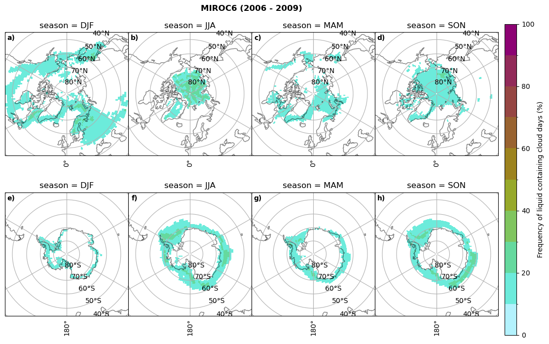
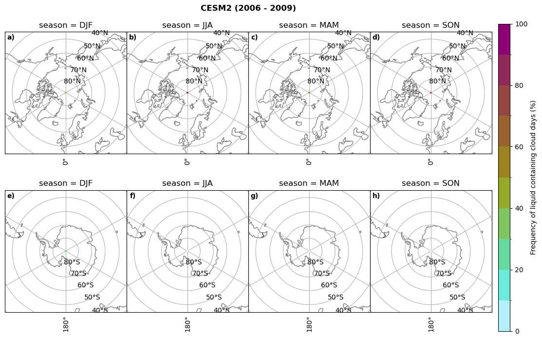
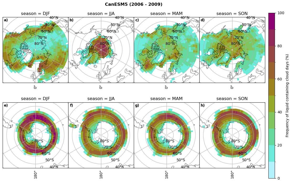
How often do we have SLC with thresholds for surface snowfall, liquid water path, and temperature

cumm = dict()
for model in dset_dict.keys():

    # create dataset with all cumm
    cumm[model] = xr.Dataset()
    # count the days per season when there was a LCC, and 2t<=0C, and where 10% per season a lcc cloud existed when also the surface temp was below freezing
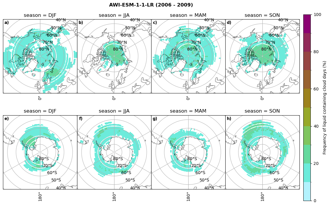
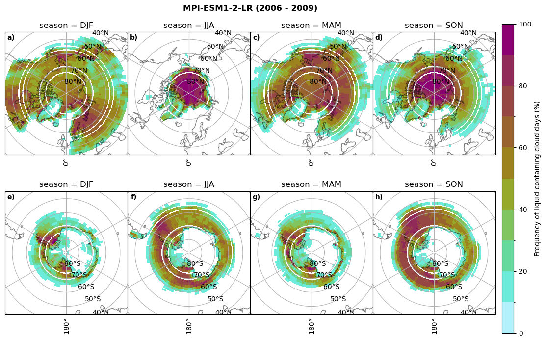
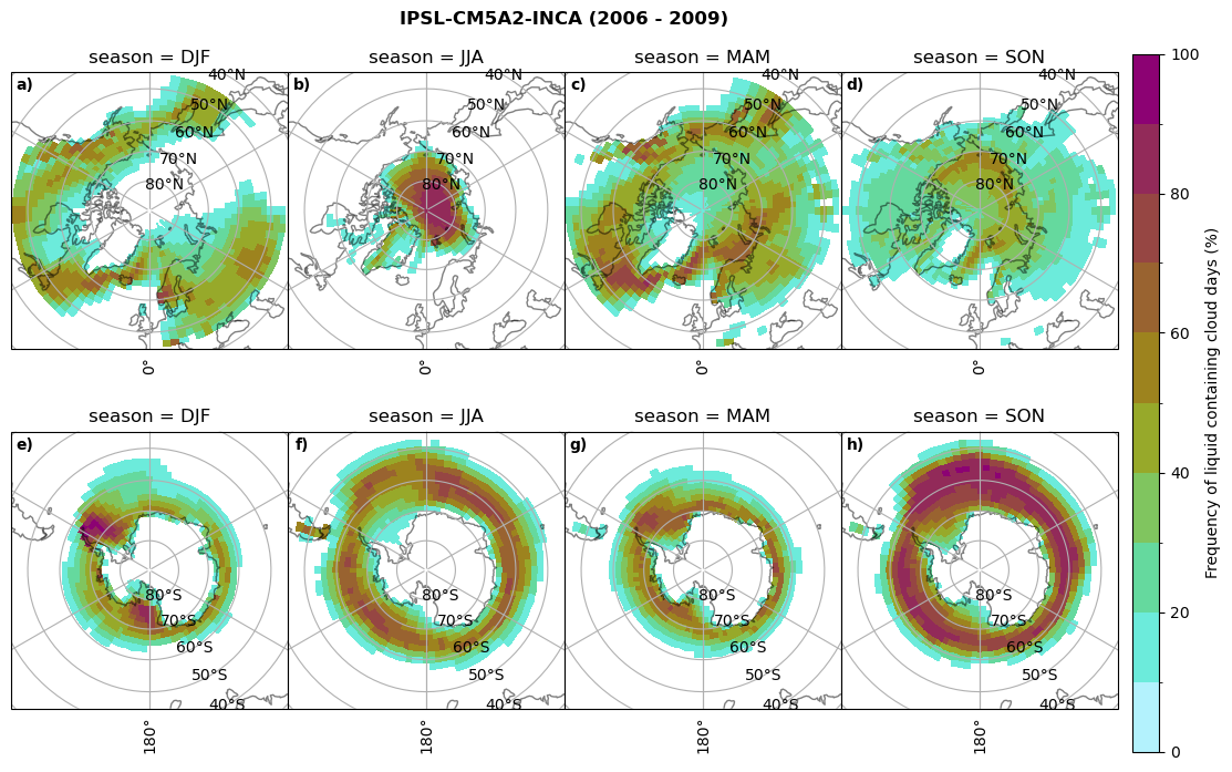
    cumm[model]['lcc_days'] = (dset_dict_lcc_2t_days[model]['twp'].groupby('time.season').count(dim='time',keep_attrs=False))/days_season
    print(model, 'min:', cumm[model]['lcc_days'].min().round(3).values,
        'max:', cumm[model]['lcc_days'].max().round(3).values,  
        'std:', cumm[model]['lcc_days'].std(skipna=True).round(3).values, 
        'mean:', cumm[model]['lcc_days'].mean(skipna=True).round(3).values)
    
        
    figname = '{}_cum_lcc_days_season_{}_{}.png'.format(model,starty, endy)
    fct.plt_seasonal_NH_SH((cumm[model]['lcc_days'].where(cumm[model]['lcc_days'] > 0.))*100, levels=np.arange(0,110,10), cbar_label='Frequency of liquid containing cloud days (%)', plt_title='{} ({} - {})'.format(model, starty,endy), extend=None)
    plt.savefig(FIG_DIR + figname, format = 'png', bbox_inches = 'tight', transparent = False)

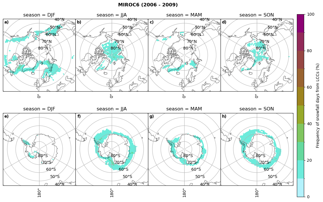
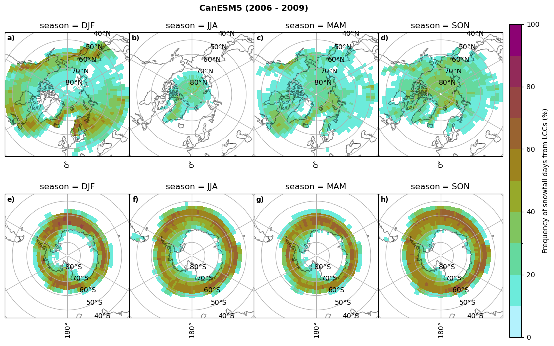
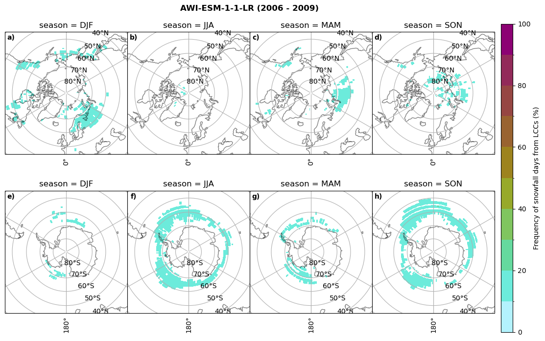
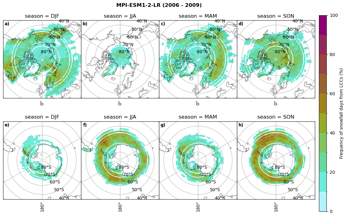
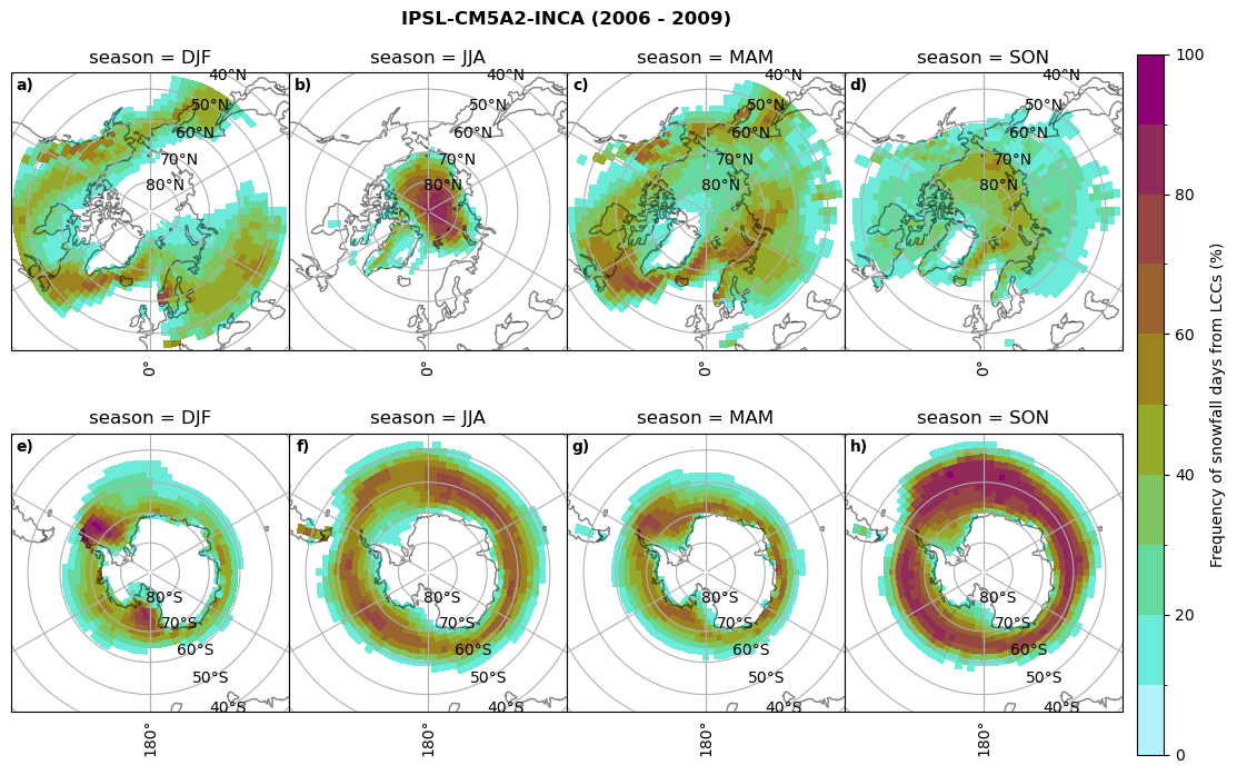
    cumm[model]['sf_days'] = (dset_dict_lcc_2t_sf_days[model]['twp'].groupby('time.season').count(dim='time',keep_attrs=False))/days_season
    print(model,'min:', cumm[model]['sf_days'].min().round(3).values,
        'max:', cumm[model]['sf_days'].max().round(3).values,  
        'std:', cumm[model]['sf_days'].std(skipna=True).round(3).values, 
        'mean:', cumm[model]['sf_days'].mean(skipna=True).round(3).values)
    figname = '{}_cum_sf_days_season_{}_{}.png'.format(model,starty, endy)
    fct.plt_seasonal_NH_SH((cumm[model]['sf_days'].where(cumm[model]['sf_days'] >0.))*100, levels=np.arange(0,110,10), cbar_label='Frequency of snowfall days from LCCs (%)', plt_title='{} ({} - {})'.format(model,starty,endy), extend=None)
    plt.savefig(FIG_DIR + figname, format = 'png', bbox_inches = 'tight', transparent = False)

MIROC6 min: 0.0 max: 0.25 std: 0.064 mean: 0.031
MIROC6 min: 0.0 max: 0.236 std: 0.043 mean: 0.014
CESM2 min: 0.0 max: 0.84 std: 0.047 mean: 0.004
CESM2 min: 0.0 max: 0.0 std: 0.0 mean: 0.0
CanESM5 min: 0.0 max: 0.928 std: 0.246 mean: 0.223
CanESM5 min: 0.0 max: 0.719 std: 0.181 mean: 0.15
AWI-ESM-1-1-LR min: 0.0 max: 0.25 std: 0.081 mean: 0.054
AWI-ESM-1-1-LR min: 0.0 max: 0.201 std: 0.027 mean: 0.006
MPI-ESM1-2-LR min: 0.0 max: 0.973 std: 0.304 mean: 0.246
MPI-ESM1-2-LR min: 0.0 max: 0.679 std: 0.138 mean: 0.098
IPSL-CM5A2-INCA min: 0.0 max: 0.931 std: 0.243 mean: 0.191
IPSL-CM5A2-INCA min: 0.0 max: 0.919 std: 0.232 mean: 0.179

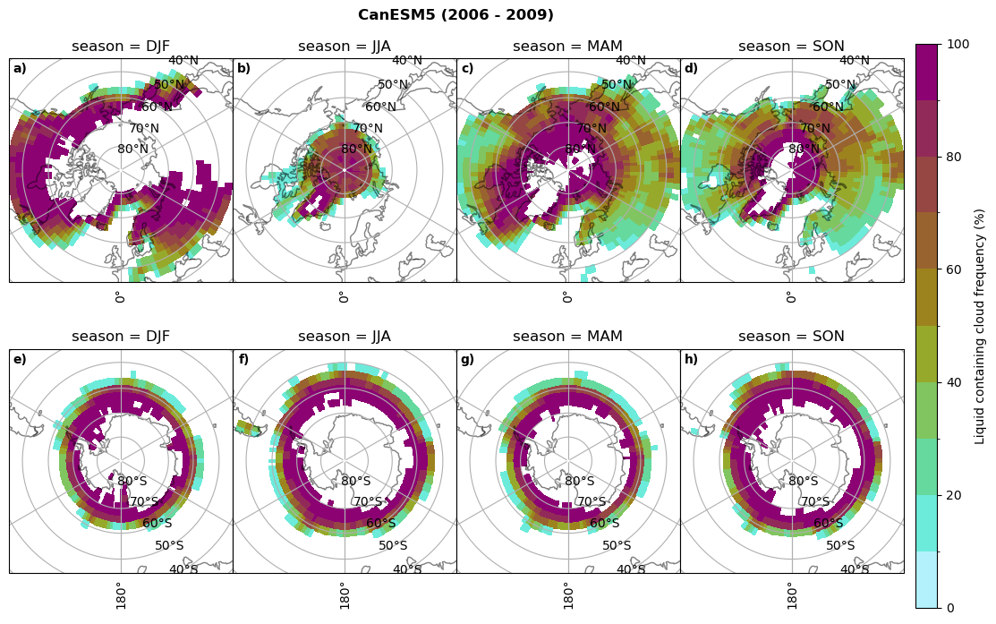
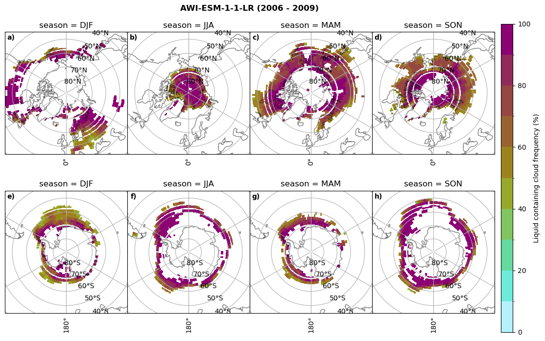
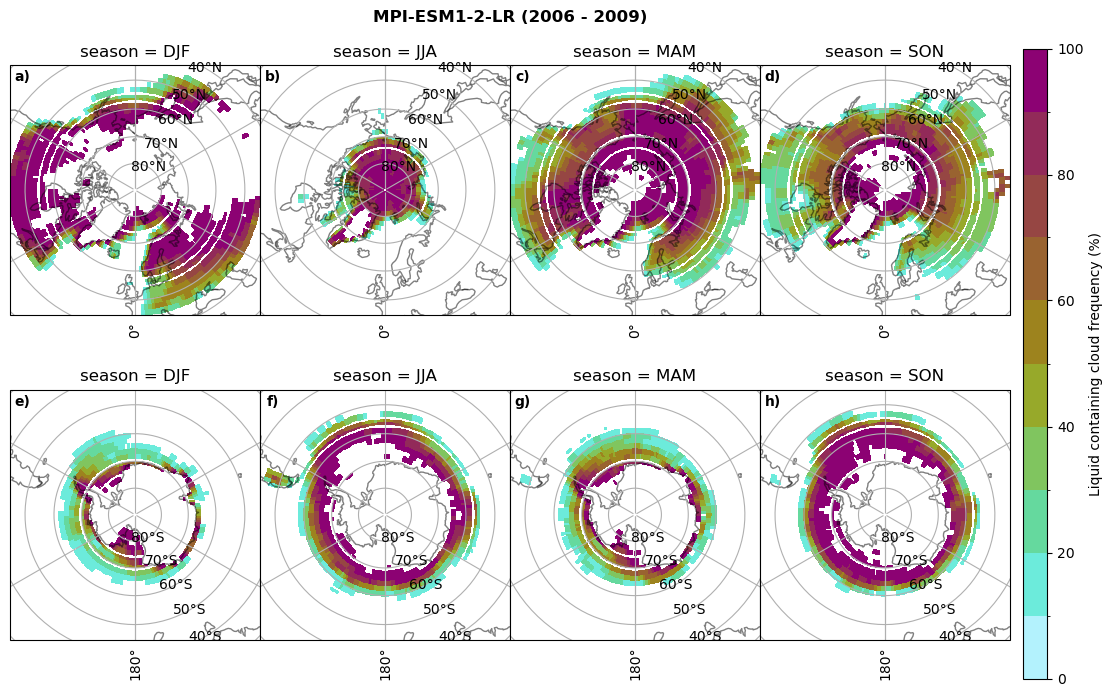
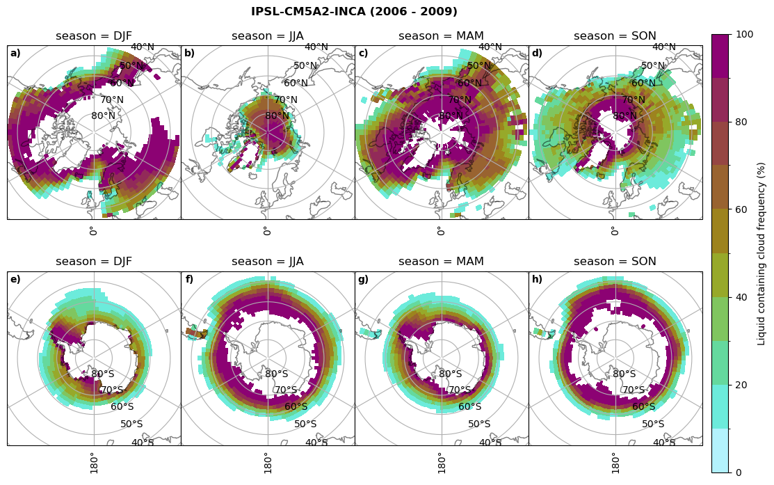
Liquid containing cloud frequency

Relative frequency

\[RF = \frac{f}{n} = \frac{\text{number of times the data occurred in an observation}}{\text{total frequency}}\]

ratios = dict()
for model in dset_dict.keys():
    ratios[model] = xr.Dataset()
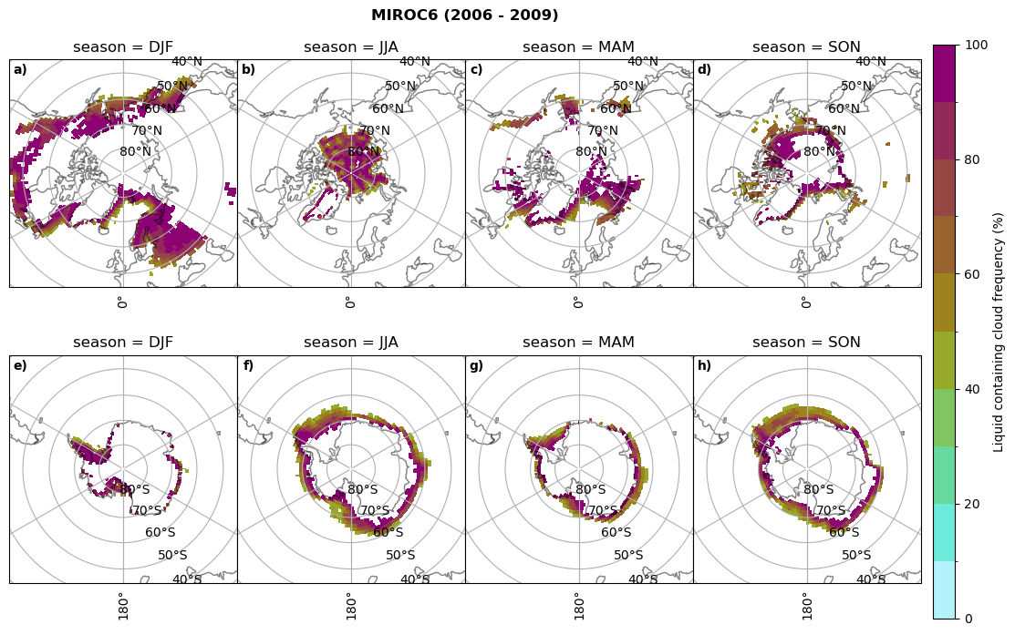
    # relative frequency of liquid containing clouds per season
    f = dset_dict_lcc_2t_days[model]['lwp'].groupby('time.season').count(dim='time', keep_attrs=False) # number of times a super cooled liquid water cloud occured when the liquid water path is larger than 5gm-2, and temperature below 0degC
    n = dset_dict_lcc[model]['lwp'].groupby('time.season').count(dim='time', keep_attrs=False)         # frequency of liquid clouds (only LWP threshold applied) when lwp is larger than 5gm-2

    ratios[model]['lcc_wo_snow_season'] = f/n

    print('min:', ratios[model]['lcc_wo_snow_season'].min().round(3).values,
        'max:', ratios[model]['lcc_wo_snow_season'].max().round(3).values,  
        'std:', ratios[model]['lcc_wo_snow_season'].std(skipna=True).round(3).values, 
        'mean:', ratios[model]['lcc_wo_snow_season'].mean(skipna=True).round(3).values)
    
    fct.plt_seasonal_NH_SH((ratios[model]['lcc_wo_snow_season'].where(ratios[model]['lcc_wo_snow_season']>0.))*100, np.arange(0,110,10), 'Liquid containing cloud frequency (%)', plt_title='{} ({} - {})'.format(model,starty,endy), extend=None)

    figname = '{}_rf_lcc_wo_snow_season_{}_{}.png'.format(model,starty, endy)
    plt.savefig(FIG_DIR + figname, format = 'png', bbox_inches = 'tight', transparent = False)

    # relative frequency of liquid containing clouds per month
    f = dset_dict_lcc_2t_days[model]['lwp'].groupby('time.month').count(dim='time', keep_attrs=False) # number of times a super cooled liquid water cloud occured when the liquid water path is larger than 5gm-2, and temperature below 0degC
    n = dset_dict_lcc[model]['lwp'].groupby('time.month').count(dim='time', keep_attrs=False)         # frequency of liquid clouds (only LWP threshold applied) when lwp is larger than 5gm-2

    ratios[model]['lcc_wo_snow_month'] = f/n

    print('min:', ratios[model]['lcc_wo_snow_month'].min().round(3).values,
        'max:', ratios[model]['lcc_wo_snow_month'].max().round(3).values,  
        'std:', ratios[model]['lcc_wo_snow_month'].std(skipna=True).round(3).values, 
        'mean:', ratios[model]['lcc_wo_snow_month'].mean(skipna=True).round(3).values)

min: 0.0 max: 1.0 std: 0.367 mean: 0.186
min: 0.0 max: 1.0 std: 0.377 mean: 0.193
min: 0.0 max: 1.0 std: 0.112 mean: 0.013
min: 0.0 max: 1.0 std: 0.113 mean: 0.013
min: 0.0 max: 1.0 std: 0.443 mean: 0.473
min: 0.0 max: 1.0 std: 0.458 mean: 0.493
min: 0.0 max: 1.0 std: 0.454 mean: 0.364
min: 0.0 max: 1.0 std: 0.466 mean: 0.379
min: 0.0 max: 1.0 std: 0.449 mean: 0.472
min: 0.0 max: 1.0 std: 0.463 mean: 0.486
min: 0.0 max: 1.0 std: 0.425 mean: 0.43
min: 0.0 max: 1.0 std: 0.447 mean: 0.449

Masked and weighted average

Make use of the xarray function weighted, but use the weights from CMIP6.

NH_mean = dict()
SH_mean = dict()
NH_std = dict()
SH_std = dict()
weights = dict()

for model in dset_dict.keys():
    NH_mean[model] = xr.Dataset()
    SH_mean[model] = xr.Dataset()

    NH_std[model] = xr.Dataset()
    SH_std[model] = xr.Dataset()

    # Grid cells have different area, so when we do the global average, they have to be weigted by the area of each grid cell.
    # weights[model] = fct.area_grid(ratios['lat'].values, ratios['lon'].values)
    weights[model] = dset_dict[model].areacella

    NH_mean[model]['lcc_wo_snow_month'] = ratios[model]['lcc_wo_snow_month'].sel(lat=slice(45,90)).weighted(weights[model].fillna(0)).mean(('lat', 'lon'))
    SH_mean[model]['lcc_wo_snow_month'] = ratios[model]['lcc_wo_snow_month'].sel(lat=slice(-90,-45)).weighted(weights[model].fillna(0)).mean(('lat', 'lon'))

    NH_std[model]['lcc_wo_snow_month'] = ratios[model]['lcc_wo_snow_month'].sel(lat=slice(45,90)).weighted(weights[model].fillna(0)).std(('lat', 'lon'))
    SH_std[model]['lcc_wo_snow_month'] = ratios[model]['lcc_wo_snow_month'].sel(lat=slice(-90,-45)).weighted(weights[model].fillna(0)).std(('lat', 'lon'))

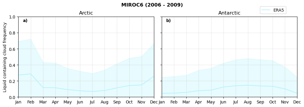
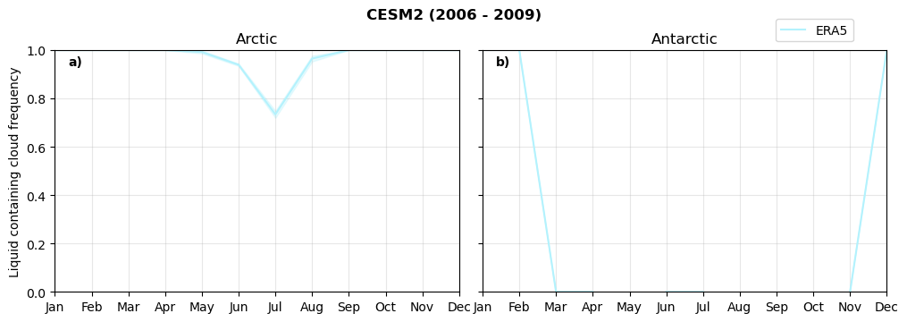
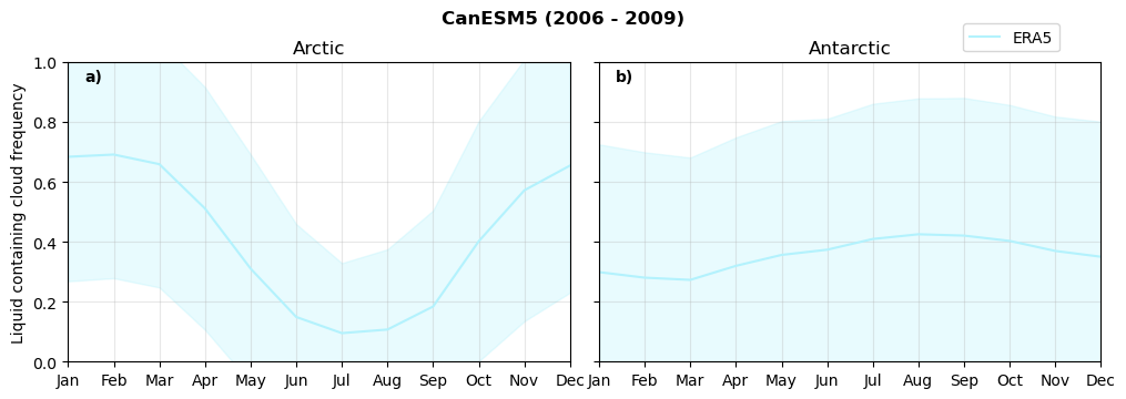
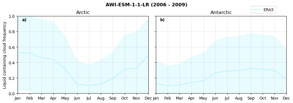
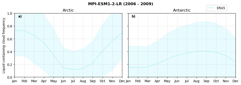
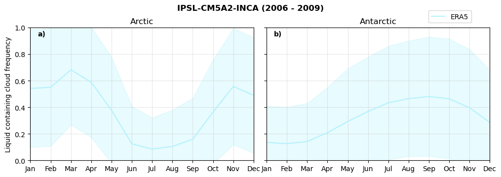
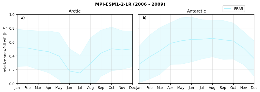
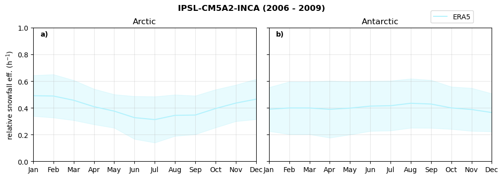
Annual cycle of frequency of liquid containing clouds

for model in dset_dict.keys():

    fct.plt_annual_cycle(NH_mean[model]['lcc_wo_snow_month'], 
                         SH_mean[model]['lcc_wo_snow_month'], 
                         NH_std[model]['lcc_wo_snow_month'], 
                         SH_std[model]['lcc_wo_snow_month'], 
                         'Liquid containing cloud frequency','{} ({} - {})'.format(model,starty,endy))
    figname = '{}_rf_lcc_wo_snow_annual_{}_{}.png'.format(model,starty, endy)
    plt.savefig(FIG_DIR + figname, format = 'png', bbox_inches = 'tight', transparent = False)

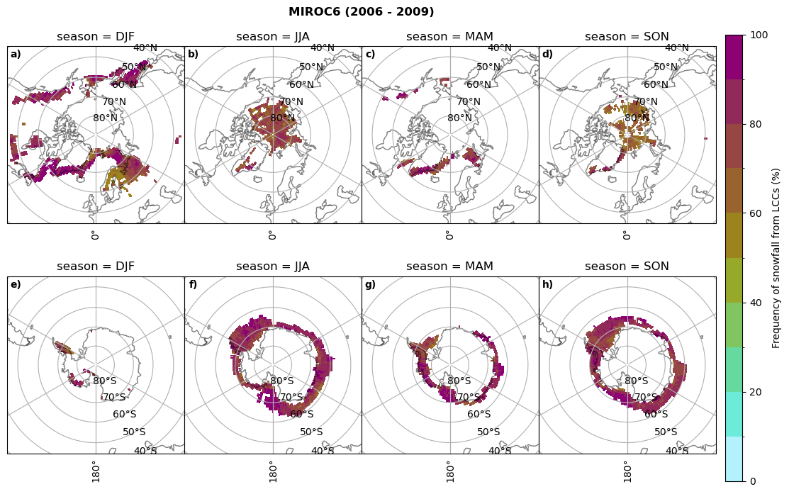
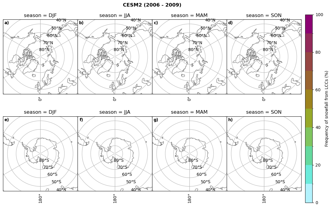
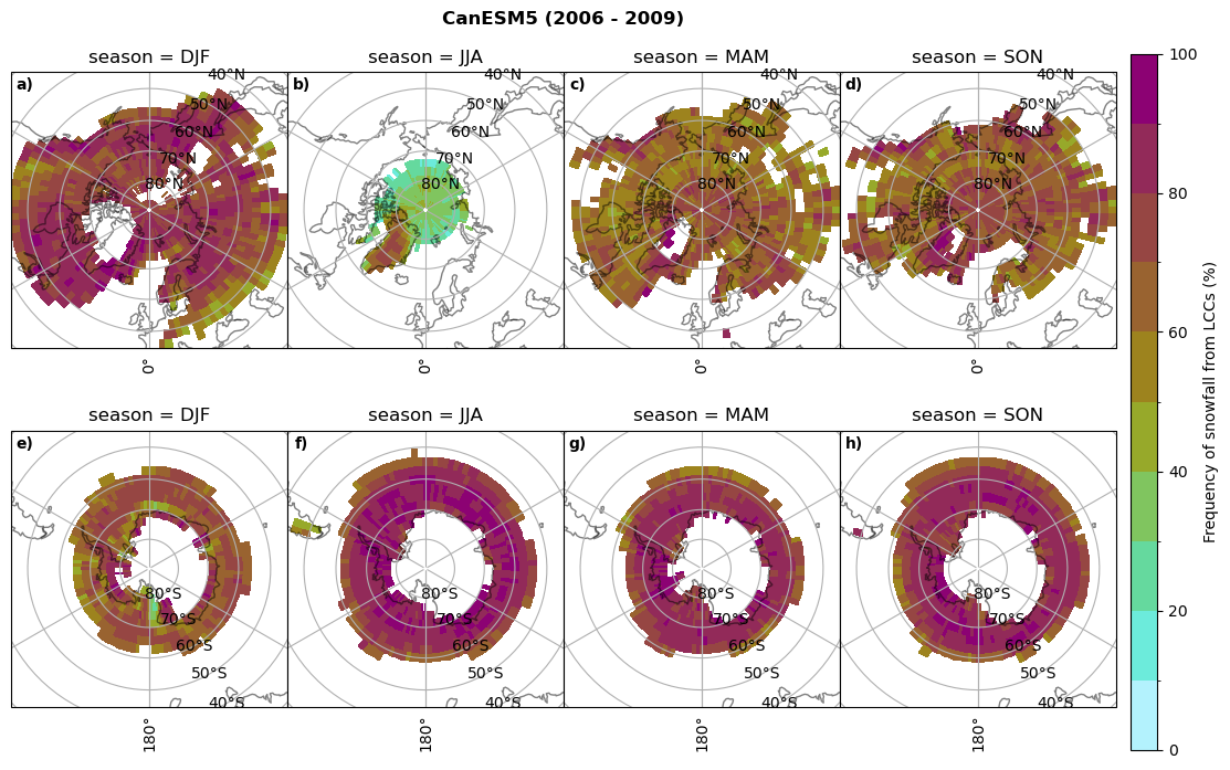
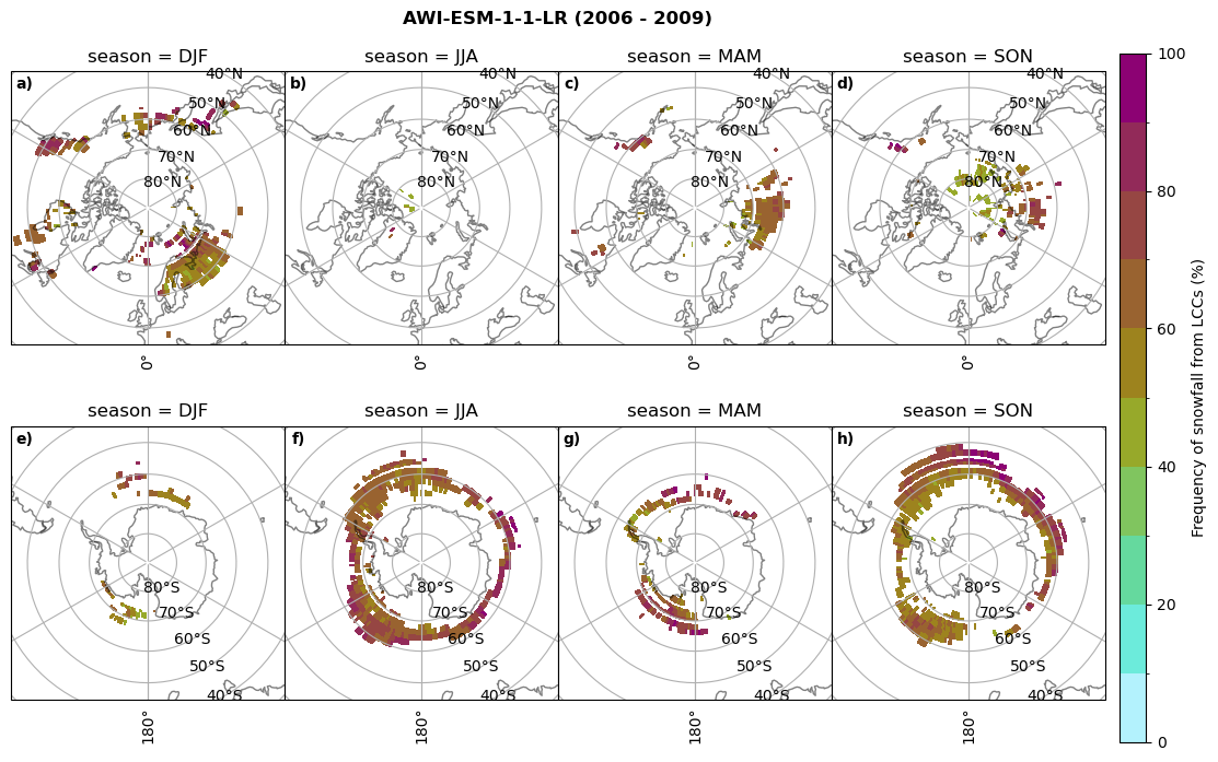
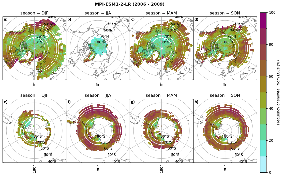
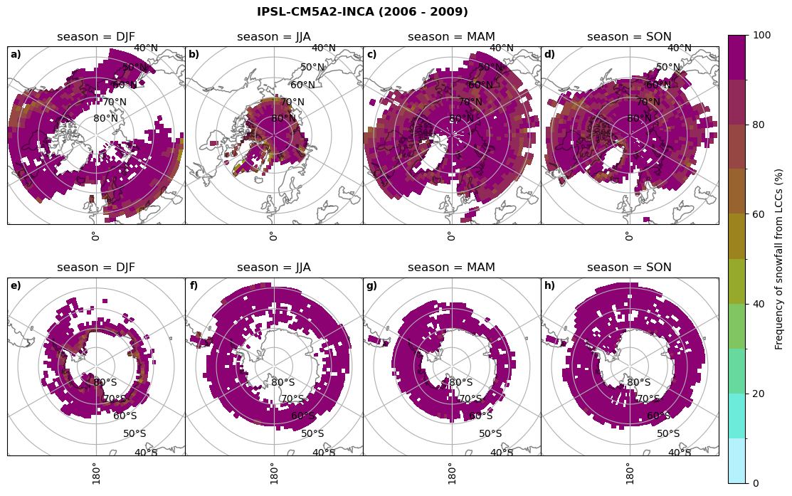
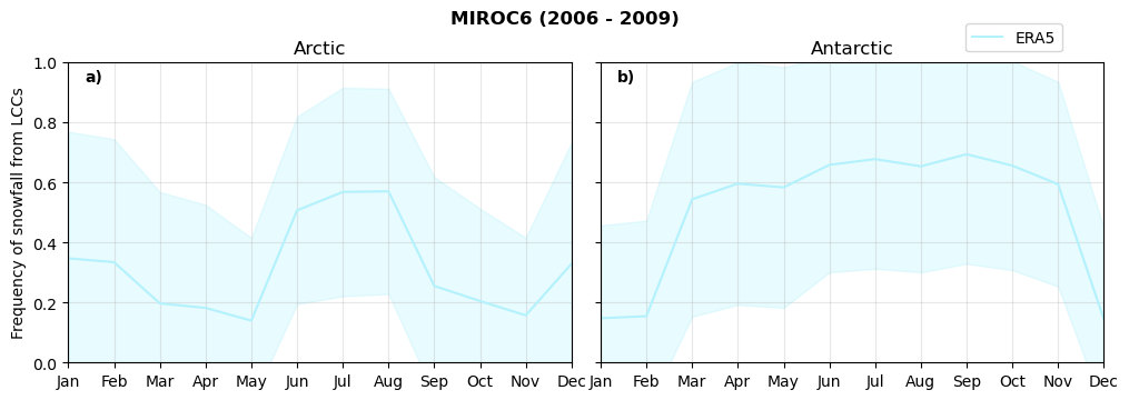
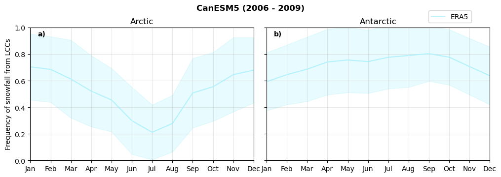
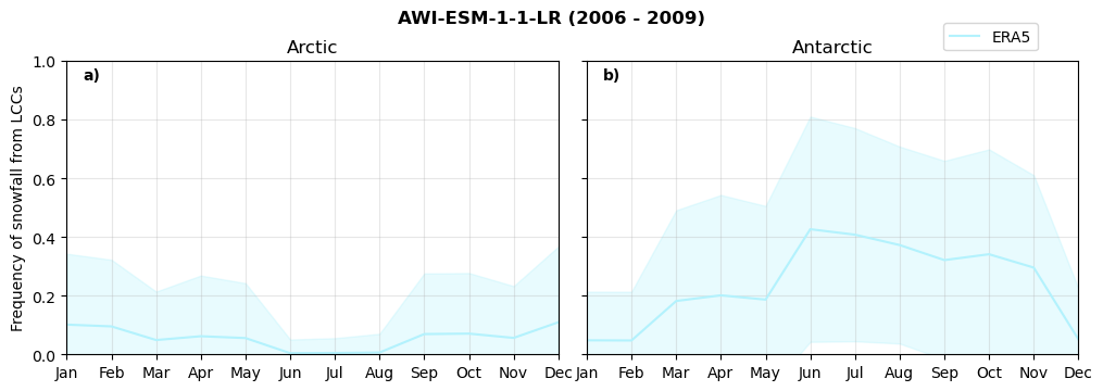
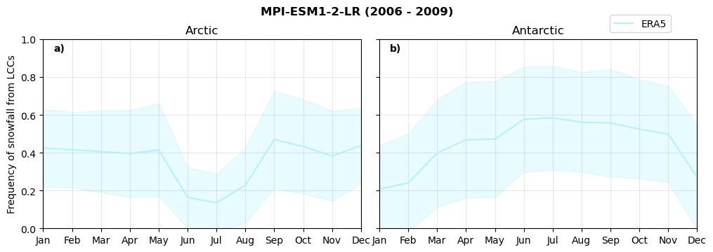
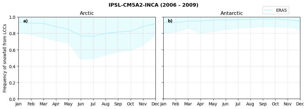
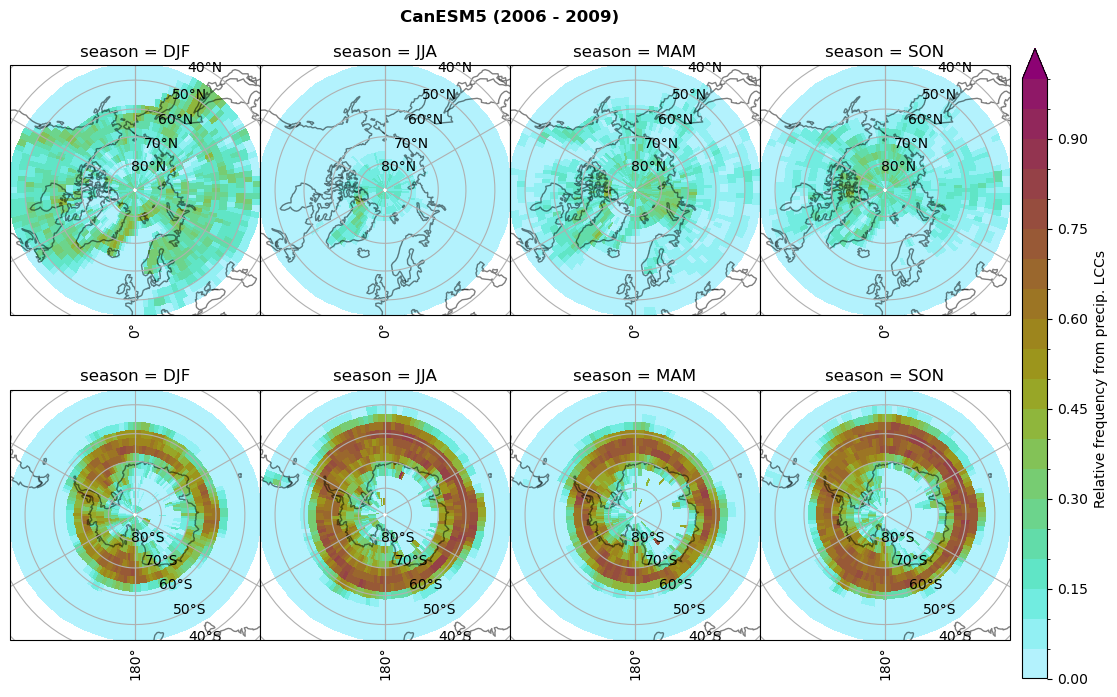
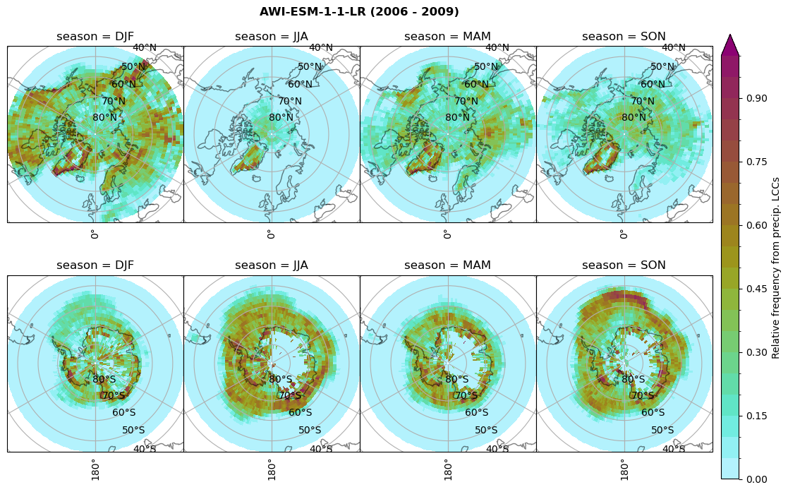
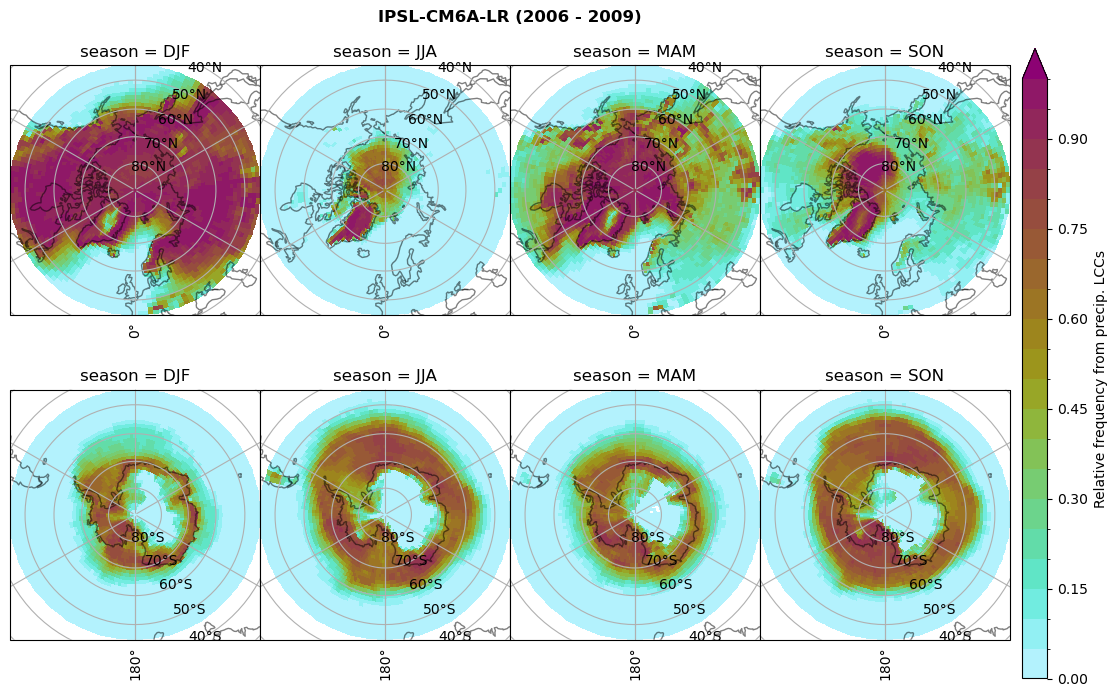
Frequency of snowfall from LCCs

for model in dset_dict.keys():

      # relative frequency of snowing liquid containing clouds per season
      f = dset_dict_lcc_2t_sf_days[model]['prsn'].groupby('time.season').count(dim='time', keep_attrs=False)  # number of times a super cooled liquid water cloud occured when the liquid water path is larger than 5gm-2, and temperature below 0degC
      n = dset_dict_lcc_2t_days[model]['lwp'].groupby('time.season').count(dim='time', keep_attrs=False)

      ratios[model]['lcc_w_snow_season'] = f/n
      print('min:', ratios[model]['lcc_w_snow_season'].min().round(3).values,
            'max:', ratios[model]['lcc_w_snow_season'].max().round(3).values,  
            'std:', ratios[model]['lcc_w_snow_season'].std(skipna=True).round(3).values, 
            'mean:', ratios[model]['lcc_w_snow_season'].mean(skipna=True).round(3).values)

      # 
      fct.plt_seasonal_NH_SH((ratios[model]['lcc_w_snow_season'].where(ratios[model]['lcc_w_snow_season']>0.))*100, np.arange(0,110,10), 'Frequency of snowfall from LCCs (%)', plt_title='{} ({} - {})'.format(model,starty,endy), extend=None)

      figname = '{}_rf_lcc_w_snow_season_{}_{}.png'.format(model,starty, endy)
      plt.savefig(FIG_DIR + figname, format = 'png', bbox_inches = 'tight', transparent = False)

      # relative frequency of liquid containing clouds per month
      f = dset_dict_lcc_2t_sf_days[model]['prsn'].groupby('time.month').count(dim='time', keep_attrs=False) # number of times a super cooled liquid water cloud occured when the liquid water path is larger than 5gm-2, and temperature below 0degC
      n = dset_dict_lcc_2t_days[model]['lwp'].groupby('time.month').count(dim='time', keep_attrs=False)         # frequency of liquid clouds (only LWP threshold applied) when lwp is larger than 5gm-2

      ratios[model]['lcc_w_snow_month'] = f/n

      print('min:', ratios[model]['lcc_w_snow_month'].min().round(3).values,
            'max:', ratios[model]['lcc_w_snow_month'].max().round(3).values,  
            'std:', ratios[model]['lcc_w_snow_month'].std(skipna=True).round(3).values, 
            'mean:', ratios[model]['lcc_w_snow_month'].mean(skipna=True).round(3).values)

      # Grid cells have different area, so when we do the global average, they have to be weigted by the area of each grid cell.
      weights[model] = dset_dict[model].areacella

      NH_mean[model]['lcc_w_snow_month'] = ratios[model]['lcc_w_snow_month'].sel(lat=slice(45,90)).weighted(weights[model].fillna(0)).mean(('lat', 'lon'))
      SH_mean[model]['lcc_w_snow_month'] = ratios[model]['lcc_w_snow_month'].sel(lat=slice(-90,-45)).weighted(weights[model].fillna(0)).mean(('lat', 'lon'))

      NH_std[model]['lcc_w_snow_month'] = ratios[model]['lcc_w_snow_month'].sel(lat=slice(45,90)).weighted(weights[model].fillna(0)).std(('lat', 'lon'))
      SH_std[model]['lcc_w_snow_month'] = ratios[model]['lcc_w_snow_month'].sel(lat=slice(-90,-45)).weighted(weights[model].fillna(0)).std(('lat', 'lon'))

min: 0.0 max: 1.0 std: 0.394 mean: 0.4
min: 0.0 max: 1.0 std: 0.398 mean: 0.394
min: 0.0 max: 0.0 std: 0.0 mean: 0.0
min: 0.0 max: 0.0 std: 0.0 mean: 0.0
min: 0.0 max: 1.0 std: 0.257 mean: 0.637
min: 0.0 max: 1.0 std: 0.272 mean: 0.64
min: 0.0 max: 1.0 std: 0.242 mean: 0.104
min: 0.0 max: 1.0 std: 0.248 mean: 0.104
min: 0.0 max: 0.981 std: 0.241 mean: 0.381
min: 0.0 max: 1.0 std: 0.252 mean: 0.381
min: 0.0 max: 1.0 std: 0.153 mean: 0.917
min: 0.0 max: 1.0 std: 0.157 mean: 0.922

Annual cycle of frequency of snowfall from LCCs

for model in dset_dict.keys():

    fct.plt_annual_cycle(NH_mean[model]['lcc_w_snow_month'], SH_mean[model]['lcc_w_snow_month'], NH_std[model]['lcc_w_snow_month'], SH_std[model]['lcc_w_snow_month'], 'Frequency of snowfall from LCCs','{} ({} - {})'.format(model,starty,endy))
    figname = '{}_rf_lcc_wo_snow_annual_{}_{}.png'.format(model,starty, endy)
    plt.savefig(FIG_DIR + figname, format = 'png', bbox_inches = 'tight', transparent = False)

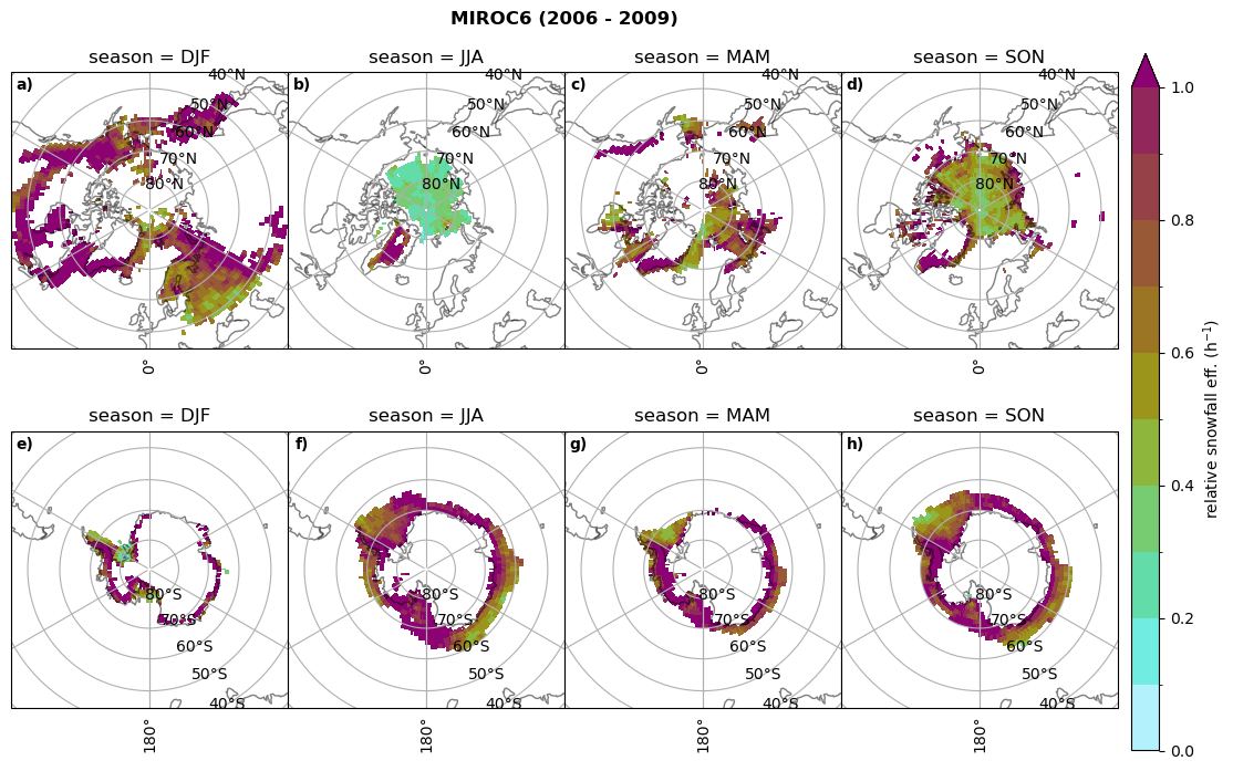
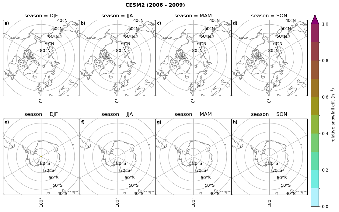
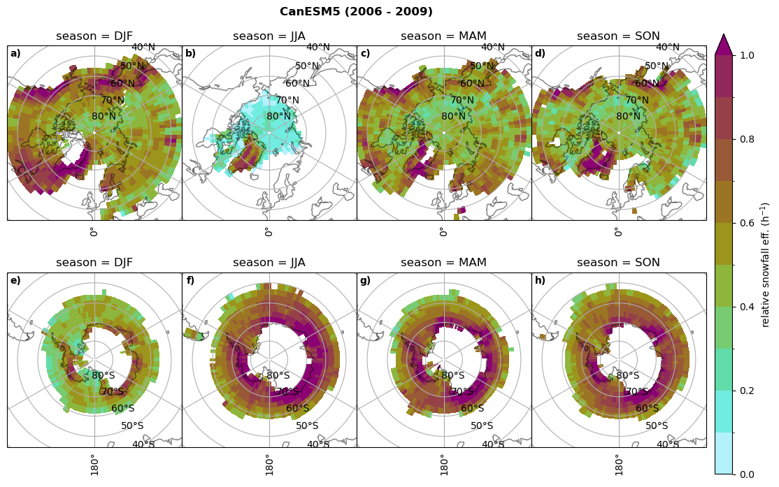
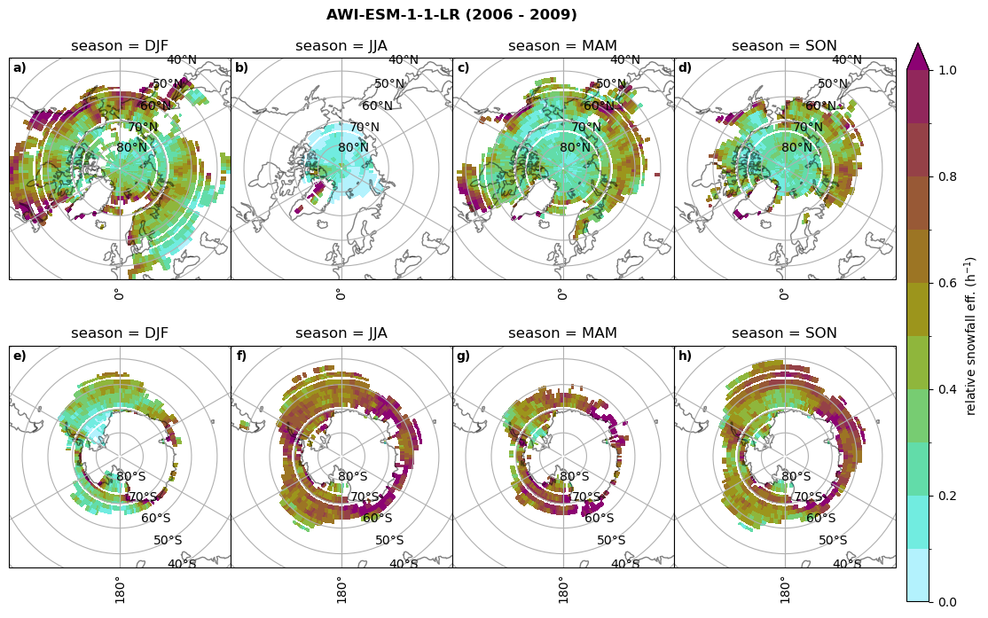
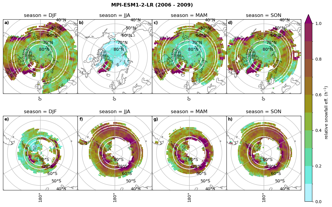
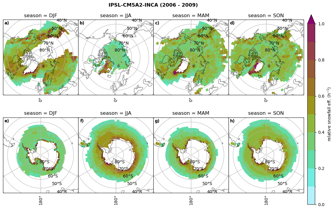
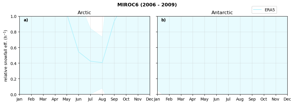
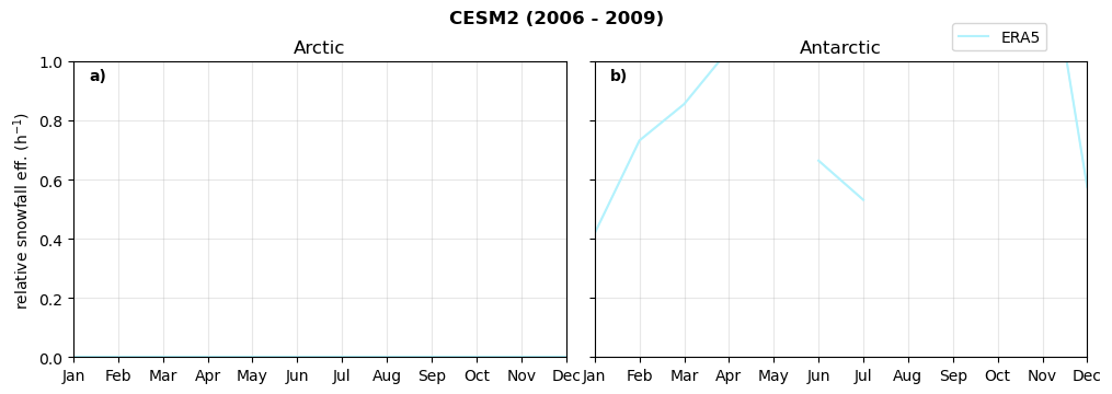
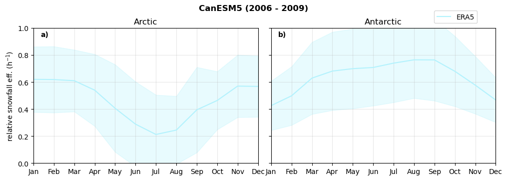
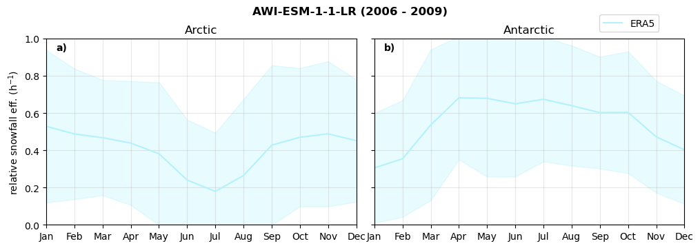
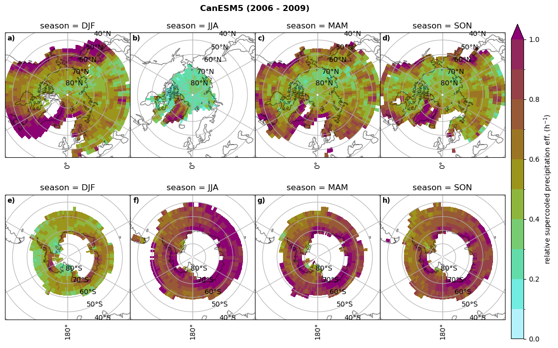
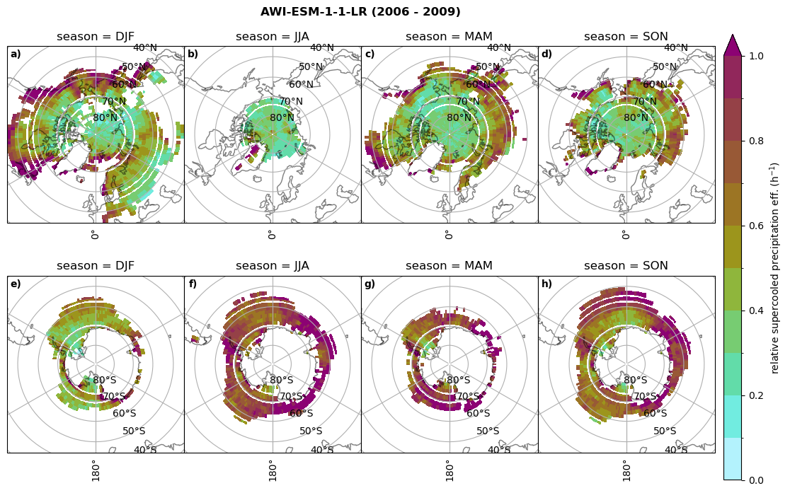
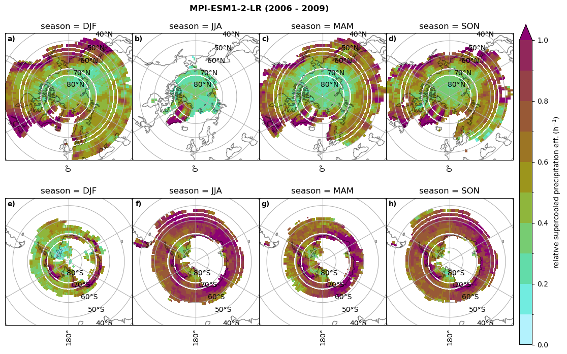
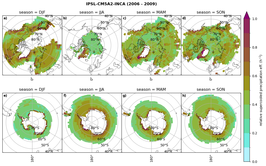
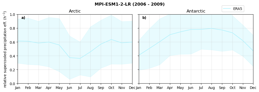
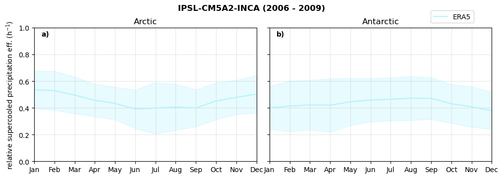
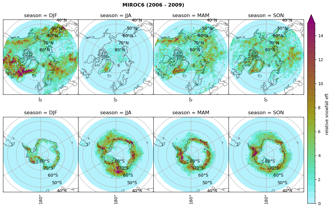
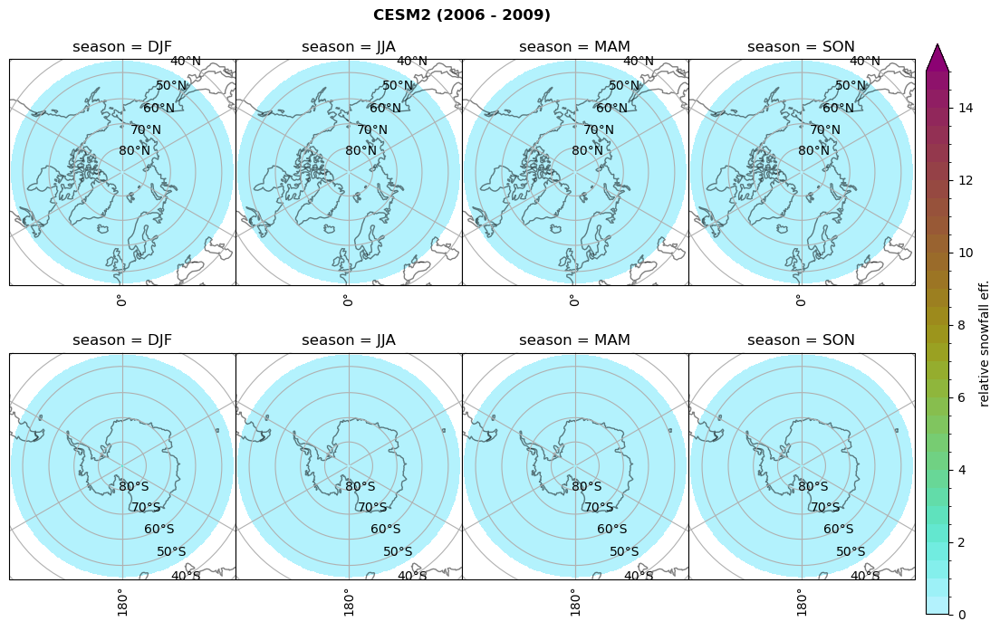
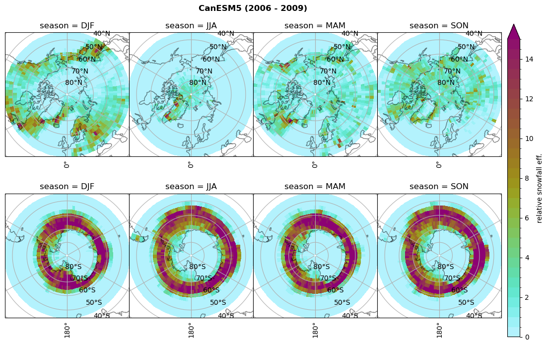
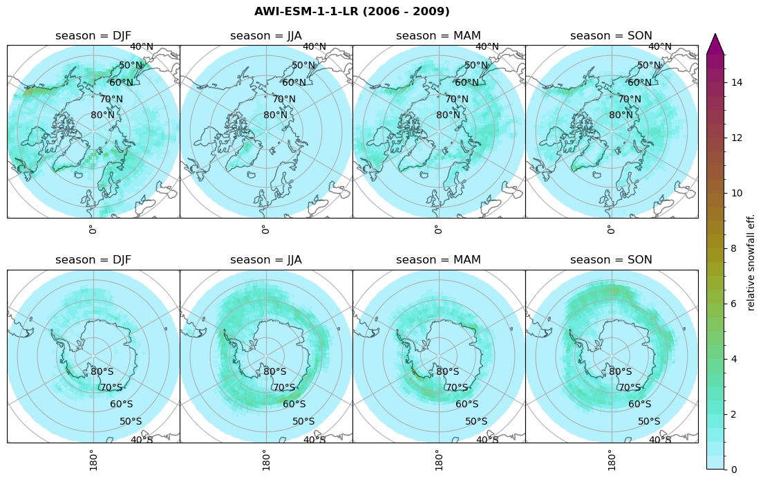
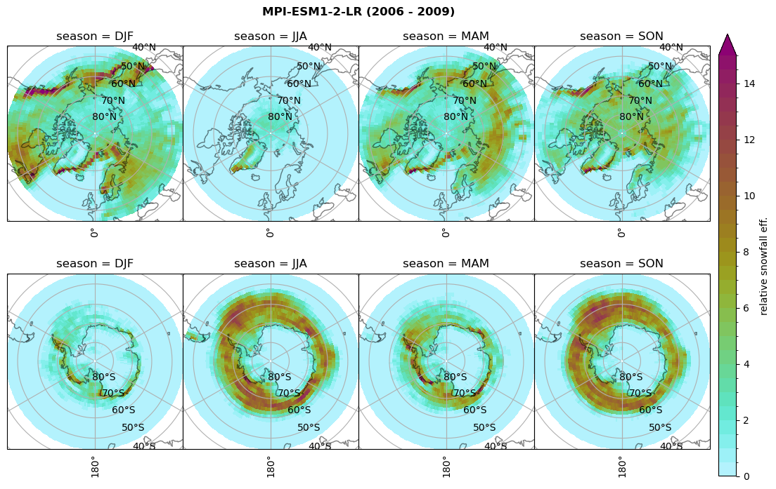
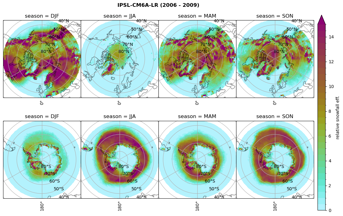
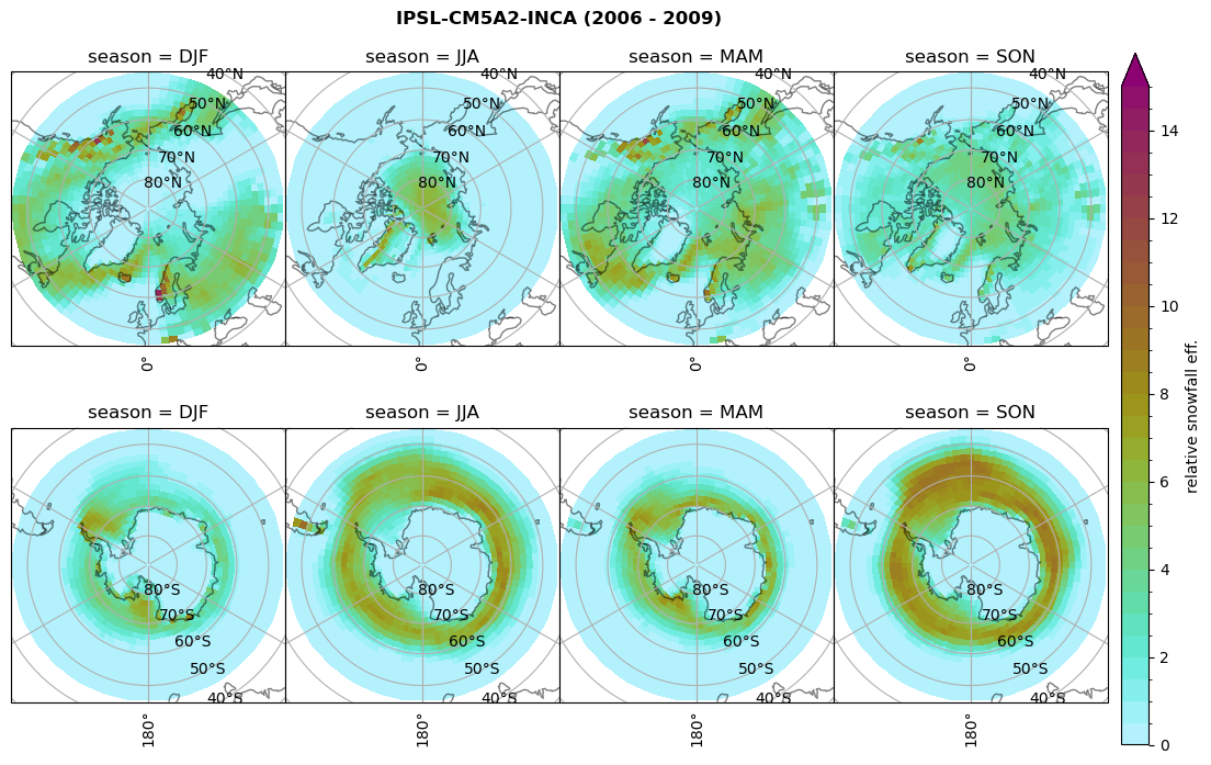
Relative snowfall efficency

The precipitation efficiency of convection is a measure of how much of the water that condenses in a rising column of air reaches the surface as precipitation [3].

In our case, we calculate the snowfall efficency by deviding the mean surface snowfall rate (sf, with units kg m-2 h-1) with the column integrated total water path (TWP, with units kg m-2). This leaves us with units of h-1, which means we get a daily mean relative snowfall efficency per hour.

\[\eta = \frac{sf}{TWP}\]

for model in dset_dict.keys():

      # snowfall efficency per season
      # first averavge over time and then fraction remove weighting only for spatial average

      ratios[model]['sf_eff_season'] = dset_dict_lcc_2t_season[model]['prsn']/dset_dict_lcc_2t_season[model]['twp']
      # plt_seasonal_NH_SH(dset_dict_lcc_2t_sf_season['prsn']/dset_dict_lcc_2t_sf_season['twp'], np.arange(0,1, 0.1),'','')
      print('min:', ratios[model]['sf_eff_season'].min().round(3).values,
            'max:', ratios[model]['sf_eff_season'].max().round(3).values,  
            'std:', ratios[model]['sf_eff_season'].std(skipna=True).round(3).values, 
            'mean:', ratios[model]['sf_eff_season'].mean(skipna=True).round(3).values)

      fct.plt_seasonal_NH_SH(ratios[model]['sf_eff_season'].where(ratios[model]['sf_eff_season']>0.), np.arange(0,1.1,0.1), 'relative snowfall eff. (h$^{-1}$)', '{} ({} - {})'.format(model, starty,endy), extend='max')
      # save precip efficency from mixed-phase clouds figure
      figname = '{}_sf_twp_season_{}_{}.png'.format(model, starty, endy)
      plt.savefig(FIG_DIR + figname, format = 'png', bbox_inches = 'tight', transparent = False)

min: 0.162 max: 6.483 std: 0.446 mean: 0.777
min: 0.557 max: 0.557 std: 0.0 mean: 0.557
min: 0.01 max: 1.745 std: 0.236 mean: 0.569
min: 0.0 max: 2.899 std: 0.262 mean: 0.425
min: 0.0 max: 2.607 std: 0.273 mean: 0.476
min: 0.14 max: 1.231 std: 0.115 mean: 0.422

Annual cycle of relative snowfall efficency

for model in dset_dict.keys():

      f = dset_dict_lcc_2t[model]['prsn'].groupby('time.month').sum(dim='time', skipna=True, keep_attrs=False)
      n = dset_dict_lcc_2t[model]['twp'].groupby('time.month').sum(dim='time', skipna=True, keep_attrs=False)
      ratios[model]['sf_eff_month'] = f/n
      NH_mean['sf_eff_month'] = ratios[model]['sf_eff_month'].sel(lat=slice(45,90)).weighted(weights[model].fillna(0)).mean(('lat', 'lon'))
      SH_mean['sf_eff_month'] = ratios[model]['sf_eff_month'].sel(lat=slice(-90,-45)).weighted(weights[model].fillna(0)).mean(('lat', 'lon'))

      NH_std['sf_eff_month'] = ratios[model]['sf_eff_month'].sel(lat=slice(45,90)).weighted(weights[model].fillna(0)).std(('lat', 'lon'))
      SH_std['sf_eff_month'] = ratios[model]['sf_eff_month'].sel(lat=slice(-90,-45)).weighted(weights[model].fillna(0)).std(('lat', 'lon'))

      print('min:', ratios[model]['sf_eff_month'].min().round(3).values,
            'max:', ratios[model]['sf_eff_month'].max().round(3).values,  
            'std:', ratios[model]['sf_eff_month'].std(skipna=True).round(3).values, 
            'mean:', ratios[model]['sf_eff_month'].mean(skipna=True).round(3).values)

      # for year in np.unique(dset_dict['time.year']):
      #     # print(year)
      #     f = dset_dict_lcc_2t['prsn'].sel(time=slice(str(year))).groupby('time.month').sum(dim='time', skipna=True, keep_attrs=False)
      #     n = dset_dict_lcc_2t['twp'].sel(time=slice(str(year))).groupby('time.month').sum(dim='time', skipna=True, keep_attrs=False)

      #     _ratio = f/n
      
      #     NH_mean['sf_eff_month_'+str(year)] = _ratio.sel(lat=slice(45,90)).weighted(weights).mean(('lat', 'lon'))
      #     SH_mean['sf_eff_month_'+str(year)] = _ratio.sel(lat=slice(-90,-45)).weighted(weights).mean(('lat', 'lon'))
      
      #     NH_std['sf_eff_month_'+str(year)] = _ratio.sel(lat=slice(45,90)).weighted(weights).std(('lat', 'lon'))
      #     SH_std['sf_eff_month_'+str(year)] = _ratio.sel(lat=slice(-90,-45)).weighted(weights).std(('lat', 'lon'))

      fct.plt_annual_cycle(NH_mean['sf_eff_month'], SH_mean['sf_eff_month'], NH_std['sf_eff_month'], SH_std['sf_eff_month'], 'relative snowfall eff. (h$^{-1}$)', '{} ({} - {})'.format(model,starty,endy))
      figname = '{}_sf_twp_annual_{}_{}.png'.format(model,starty, endy)
      plt.savefig(FIG_DIR + figname, format = 'png', bbox_inches = 'tight', transparent = False)

min: 0.0 max: 84.79 std: 1.97 mean: 1.357
min: 0.0 max: 1.504 std: 0.438 mean: 0.316
min: 0.0 max: 5.067 std: 0.284 mean: 0.557
min: 0.0 max: 4.663 std: 0.35 mean: 0.453
min: 0.0 max: 3.122 std: 0.301 mean: 0.464
min: 0.0 max: 1.769 std: 0.172 mean: 0.437

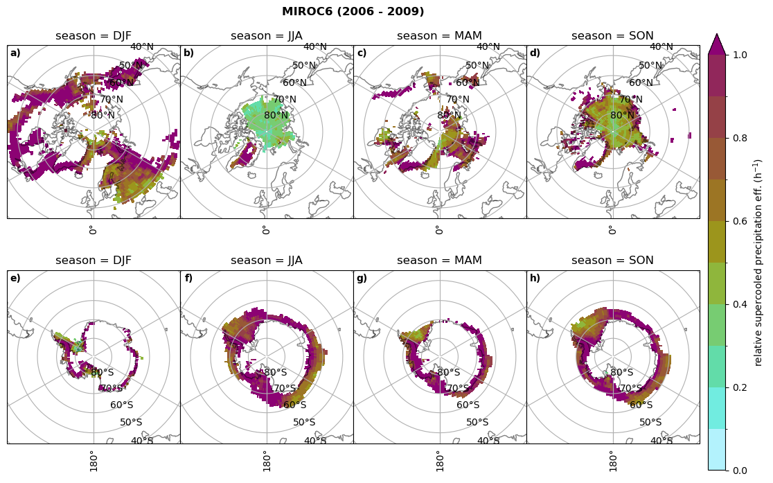
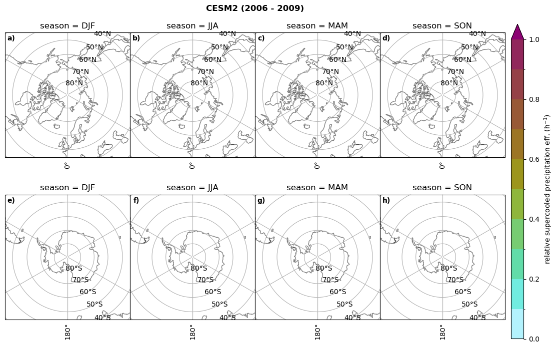
Relative precipitation efficency

Use of total precipitation, but where LWP \(\ge\) 0.005 gm-2, 2-meter temperature \(\le\) 273.15K.

for model in dset_dict.keys():

      # supercooled precipitation efficency per season
      # first averavge over time and then fraction remove weighting only for spatial average

      ratios[model]['tp_eff_season'] = dset_dict_lcc_2t_season[model]['pr']/dset_dict_lcc_2t_season[model]['twp']
      # plt_seasonal_NH_SH(dset_dict_lcc_2t_tp_season['msr']/dset_dict_lcc_2t_tp_season['twp'], np.arange(0,1, 0.1),'','')
      print('min:', ratios[model]['tp_eff_season'].min().round(3).values,
            'max:', ratios[model]['tp_eff_season'].max().round(3).values,  
            'std:', ratios[model]['tp_eff_season'].std(skipna=True).round(3).values, 
            'mean:', ratios[model]['tp_eff_season'].mean(skipna=True).round(3).values)

      # Plot precipitation efficency

      fct.plt_seasonal_NH_SH(ratios[model]['tp_eff_season'].where(ratios[model]['tp_eff_season'] >0.), np.arange(0,1.1,0.1), 'relative supercooled precipitation eff. (h$^{-1}$)', '{} ({} - {})'.format(model, starty,endy), extend='max')
      # save precip efficency from mixed-phase clouds figure
      figname = '{}_tp_twp_season_{}_{}.png'.format(model, starty, endy)
      plt.savefig(FIG_DIR + figname, format = 'png', bbox_inches = 'tight', transparent = False)

min: 0.178 max: 6.485 std: 0.445 mean: 0.799
min: nan max: nan std: nan mean: nan
min: 0.115 max: 1.88 std: 0.248 mean: 0.633
min: 0.09 max: 3.051 std: 0.265 mean: 0.531
min: 0.117 max: 2.692 std: 0.273 mean: 0.581
min: 0.212 max: 1.231 std: 0.111 mean: 0.454

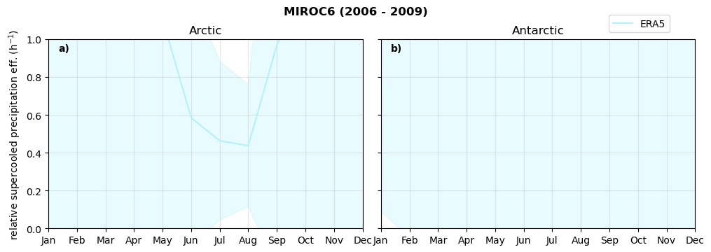
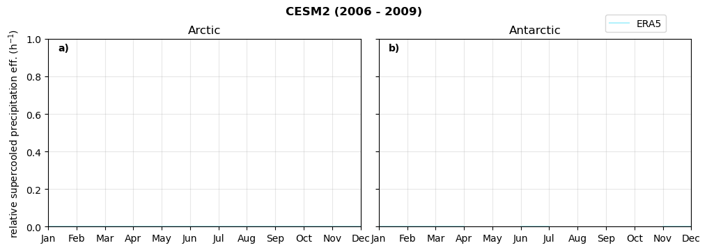
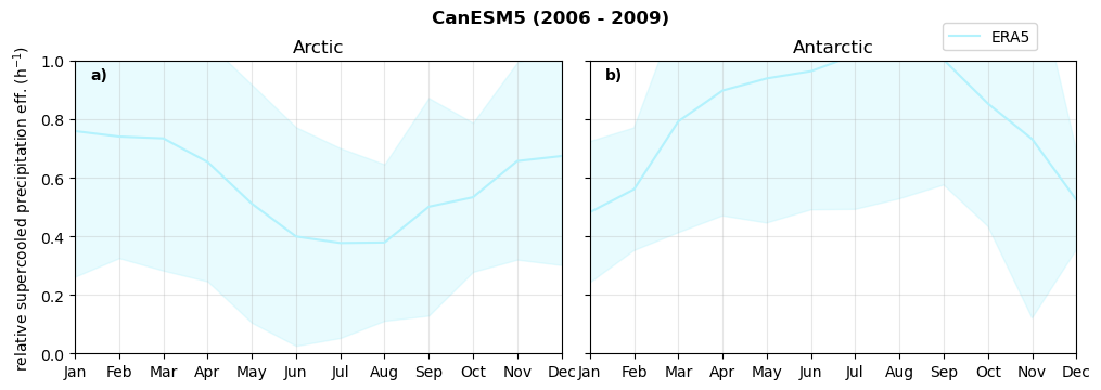
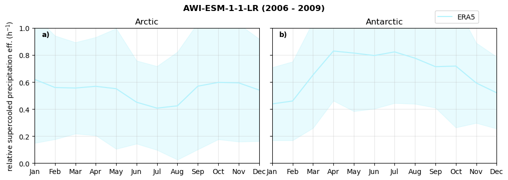
Annual cycle of relative supercooled precipitation efficency

for model in dset_dict.keys():

      f = dset_dict_lcc_2t[model]['pr'].groupby('time.month').sum(dim='time', skipna=True, keep_attrs=False)
      n = dset_dict_lcc_2t[model]['twp'].groupby('time.month').sum(dim='time', skipna=True, keep_attrs=False)
      ratios[model]['tp_eff_month'] = f/n
      NH_mean[model]['tp_eff_month'] = ratios[model]['tp_eff_month'].sel(lat=slice(45,90)).weighted(weights[model].fillna(0)).mean(('lat', 'lon'))
      SH_mean[model]['tp_eff_month'] = ratios[model]['tp_eff_month'].sel(lat=slice(-90,-45)).weighted(weights[model].fillna(0)).mean(('lat', 'lon'))

      NH_std[model]['tp_eff_month'] = ratios[model]['tp_eff_month'].sel(lat=slice(45,90)).weighted(weights[model].fillna(0)).std(('lat', 'lon'))
      SH_std[model]['tp_eff_month'] = ratios[model]['tp_eff_month'].sel(lat=slice(-90,-45)).weighted(weights[model].fillna(0)).std(('lat', 'lon'))

      print('min:', ratios[model]['tp_eff_month'].min().round(3).values,
            'max:', ratios[model]['tp_eff_month'].max().round(3).values,  
            'std:', ratios[model]['tp_eff_month'].std(skipna=True).round(3).values, 
            'mean:', ratios[model]['tp_eff_month'].mean(skipna=True).round(3).values)
      # for year in np.unique(dset_dict['time.year']):
      #     # print(year)
      #     f = dset_dict_lcc_2t[model]['pr'].sel(time=slice(str(year))).groupby('time.month').sum(dim='time', skipna=True, keep_attrs=False)
      #     n = dset_dict_lcc_2t[model]['twp'].sel(time=slice(str(year))).groupby('time.month').sum(dim='time', skipna=True, keep_attrs=False)

      #     _ratio = f/n
      
      #     NH_mean[model]['tp_eff_month_'+str(year)] = _ratio.sel(lat=slice(45,90)).weighted(weights[model]).mean(('lat', 'lon'))
      #     SH_mean[model]['tp_eff_month_'+str(year)] = _ratio.sel(lat=slice(-90,-45)).weighted(weights[model]).mean(('lat', 'lon'))
      
      #     NH_std[model]['tp_eff_month_'+str(year)] = _ratio.sel(lat=slice(45,90)).weighted(weights[model]).std(('lat', 'lon'))
      #     SH_std[model]['tp_eff_month_'+str(year)] = _ratio.sel(lat=slice(-90,-45)).weighted(weights[model]).std(('lat', 'lon'))

      fct.plt_annual_cycle(NH_mean[model]['tp_eff_month'], SH_mean[model]['tp_eff_month'], NH_std[model]['tp_eff_month'], SH_std[model]['tp_eff_month'], 'relative supercooled precipitation eff. (h$^{-1}$)', '{} ({} - {})'.format(model,starty,endy))
      figname = '{}_tp_twp_annual_{}_{}.png'.format(model,starty, endy)
      plt.savefig(FIG_DIR + figname, format = 'png', bbox_inches = 'tight', transparent = False)

min: 0.014 max: 84.796 std: 1.971 mean: 1.381
min: 0.0 max: 0.0 std: 0.0 mean: 0.0
min: 0.0 max: 9.465 std: 0.398 mean: 0.658
min: 0.0 max: 12.083 std: 0.367 mean: 0.556
min: 0.0 max: 6.72 std: 0.307 mean: 0.568
min: 0.0 max: 1.833 std: 0.161 mean: 0.467

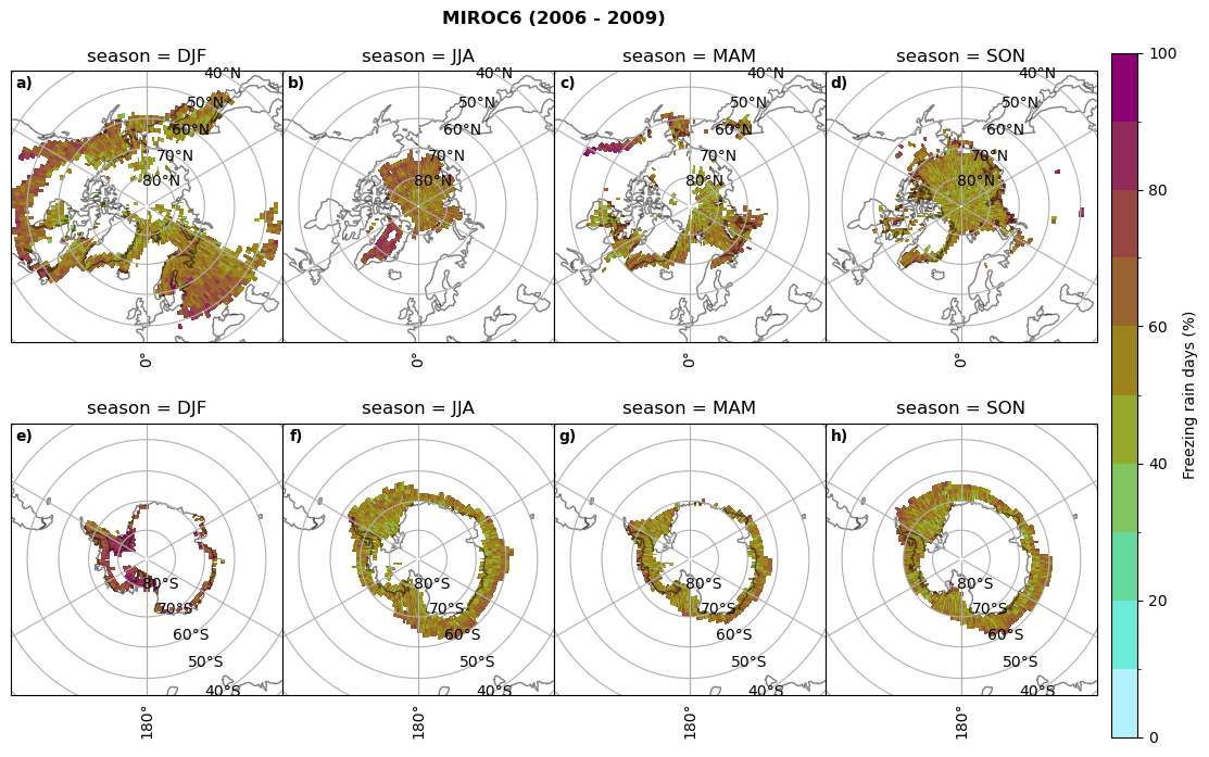
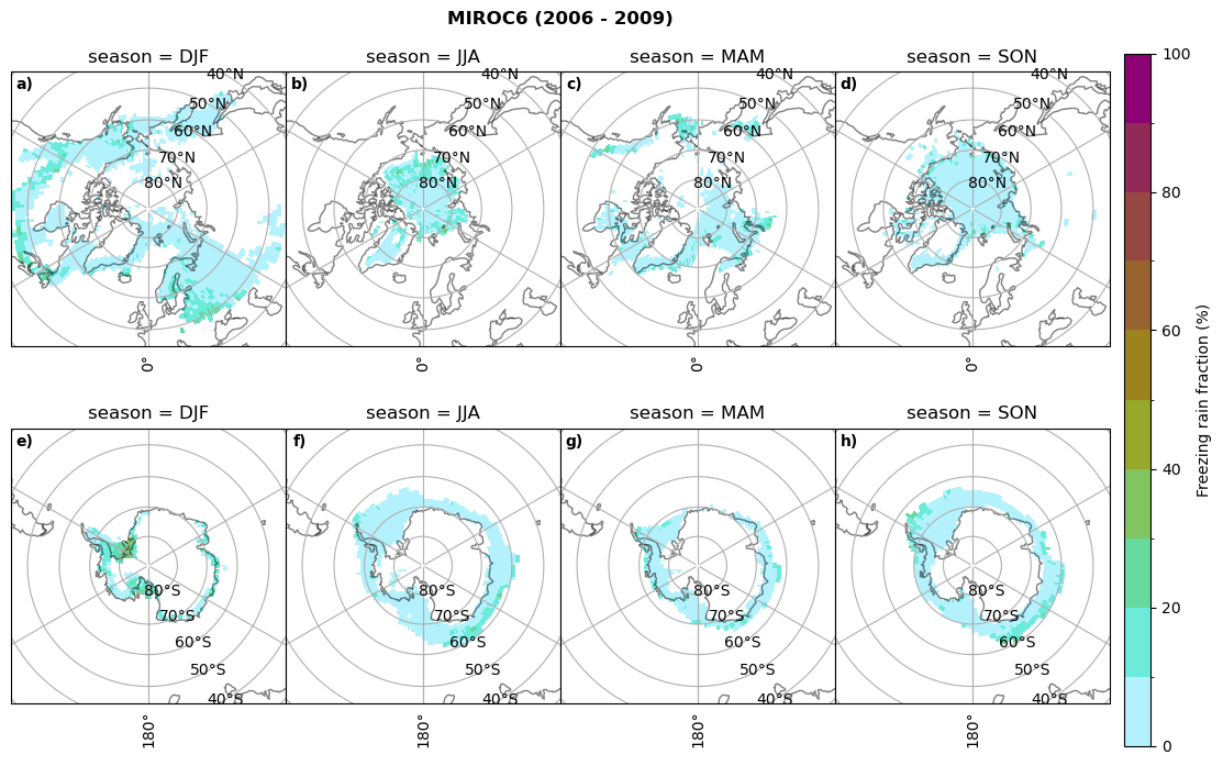
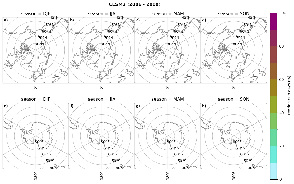
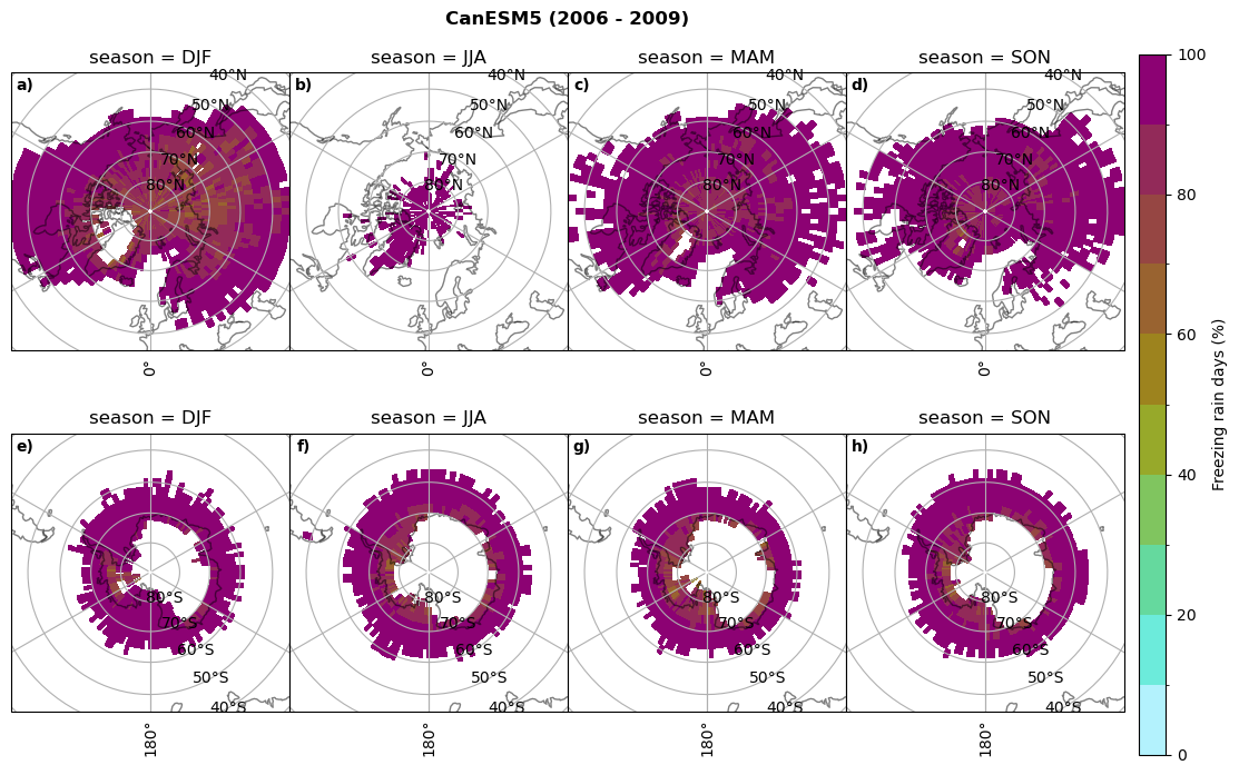
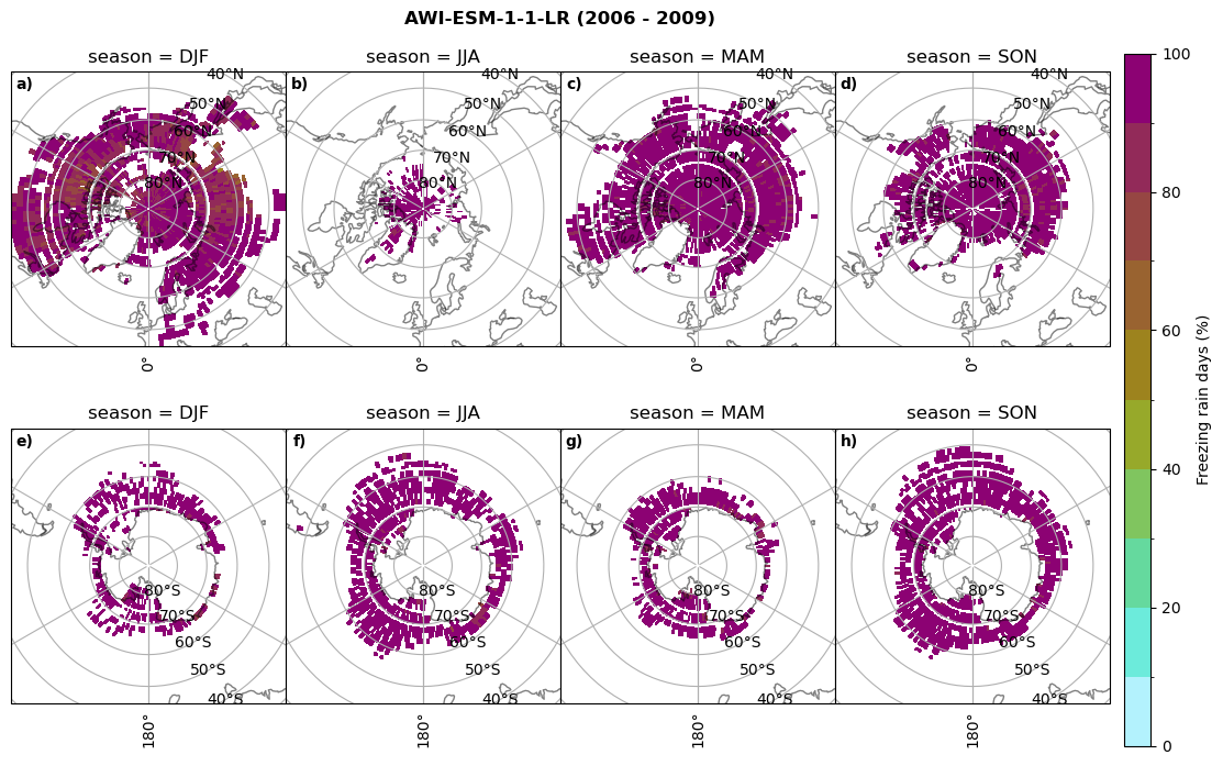
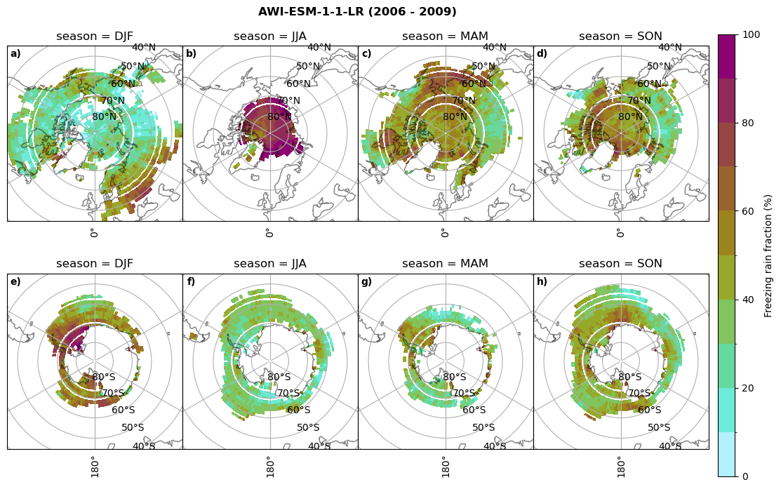
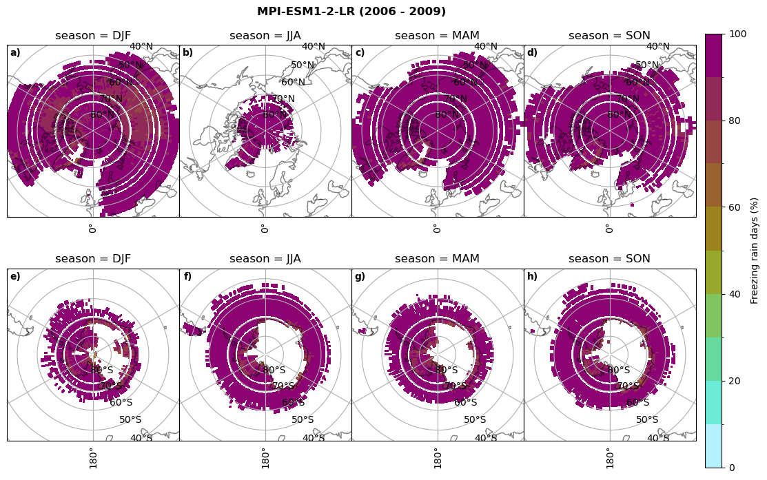
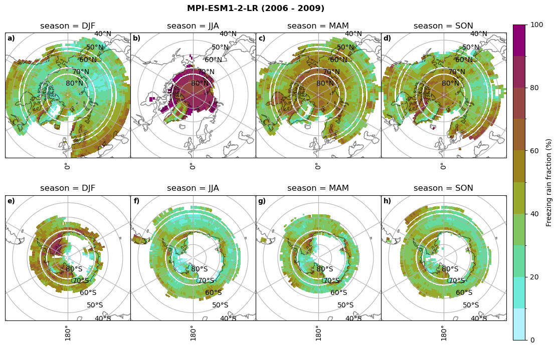
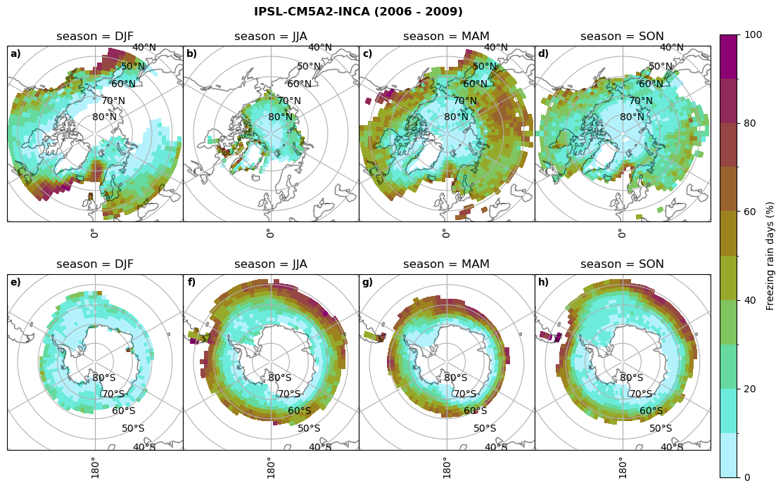
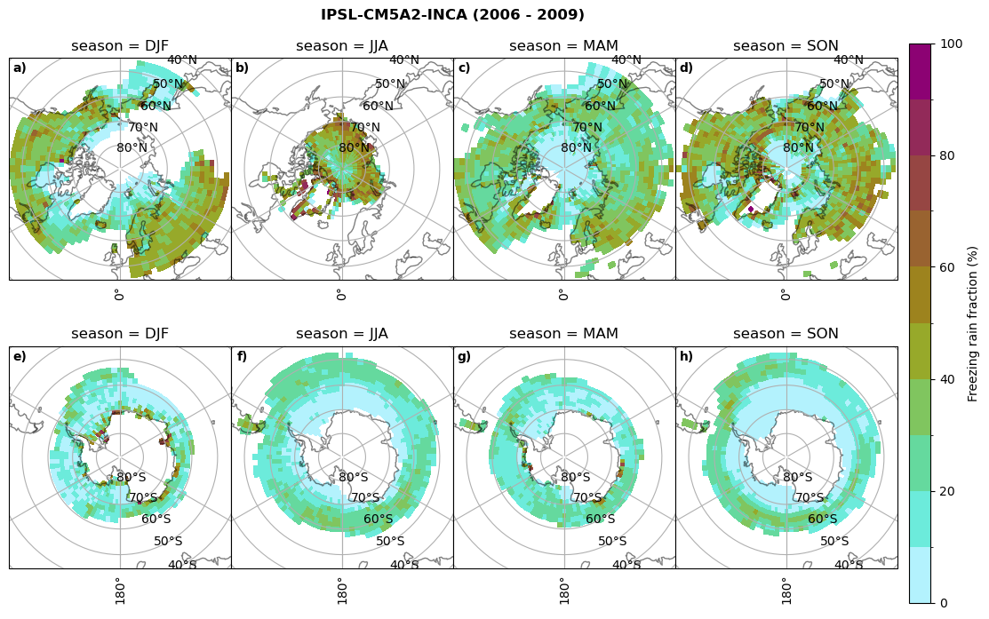
Frequency of freezing rain

Use of the thresholds.

\[RF = \frac{\text{total precipitation}(T\le273.15; LWP\ge0.005gm^{-2}) - \text{snowfall}(T\le273.15; LWP\ge0.005gm^{-2})}{\text{total precipitation}(T\le273.15; LWP\ge0.005gm^{-2})}\]

for model in dset_dict.keys():

      # first count the days where we have freezing rain per season and relate to total precipitation days
      fr_d = dset_dict_lcc_2t_days[model]['mfrr'].where(dset_dict_lcc_2t_days[model]['mfrr']>0.).groupby('time.season').count('time',keep_attrs=False)
      tp_d = dset_dict_lcc_2t_days[model]['pr'].where(dset_dict_lcc_2t_days[model]['pr']>0.).groupby('time.season').count('time',keep_attrs=False)

      ratios[model]['mfrr_pr_days'] = fr_d/tp_d

      print('min:', ratios[model]['mfrr_pr_days'].min().round(3).values,
            'max:', ratios[model]['mfrr_pr_days'].max().round(3).values,  
            'std:', ratios[model]['mfrr_pr_days'].std(skipna=True).round(3).values, 
            'mean:', ratios[model]['mfrr_pr_days'].mean(skipna=True).round(3).values)

      fct.plt_seasonal_NH_SH(ratios[model]['mfrr_pr_days'].where(ratios[model]['mfrr_pr_days']>0)*100, np.arange(0,110,10), 'Freezing rain days (%)', '{} ({} - {})'.format(model,starty,endy), extend=None)
      figname = '{}_mfrr_mtpr_days_{}_{}.png'.format(model,starty, endy)
      plt.savefig(FIG_DIR + figname, format = 'png', bbox_inches = 'tight', transparent = False)

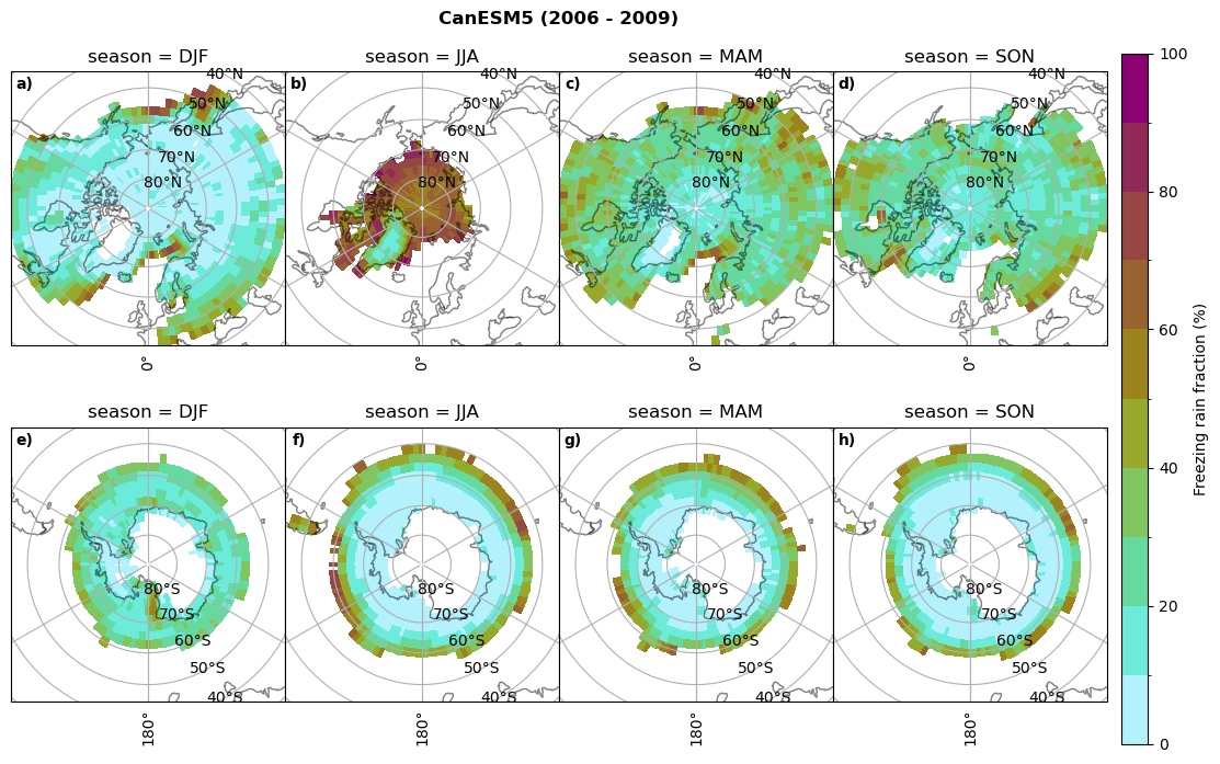
      # then bring the amount of freezing rain into relation to the total precipitation (How many percent is freezing rain in comparison to total precipitation)
      fr = dset_dict_lcc_2t_days[model]['mfrr'].where(dset_dict_lcc_2t_days[model]['mfrr']>0.)
      tp = dset_dict_lcc_2t_days[model]['pr'].where(dset_dict_lcc_2t_days[model]['pr']>0.)

      ratios[model]['mfrr_pr_frac'] = (fr/tp).groupby('time.season').mean('time',skipna=True,keep_attrs=False)
      print('min:', ratios[model]['mfrr_pr_frac'].min().round(3).values,
            'max:', ratios[model]['mfrr_pr_frac'].max().round(3).values,  
            'std:', ratios[model]['mfrr_pr_frac'].std(skipna=True).round(3).values, 
            'mean:', ratios[model]['mfrr_pr_frac'].mean(skipna=True).round(3).values)

      fct.plt_seasonal_NH_SH(ratios[model]['mfrr_pr_frac'].where(ratios[model]['mfrr_pr_frac']>0)*100, np.arange(0,110,10), 'Freezing rain fraction (%)', '{} ({} - {})'.format(model,starty,endy), extend=None)
      figname = '{}_mfrr_mtpr_amount_season_{}_{}.png'.format(model,starty, endy)
      plt.savefig(FIG_DIR + figname, format = 'png', bbox_inches = 'tight', transparent = False)

min: 0.268 max: 0.972 std: 0.101 mean: 0.573
min: 0.0 max: 0.381 std: 0.054 mean: 0.05
min: nan max: nan std: nan mean: nan
min: nan max: nan std: nan mean: nan
min: 0.568 max: 1.0 std: 0.072 mean: 0.932
min: 0.0 max: 0.918 std: 0.182 mean: 0.224
min: 0.595 max: 1.0 std: 0.046 mean: 0.958
min: 0.03 max: 1.0 std: 0.188 mean: 0.463
min: 0.509 max: 1.0 std: 0.052 mean: 0.947
min: 0.015 max: 1.0 std: 0.174 mean: 0.447
min: 0.0 max: 0.977 std: 0.19 mean: 0.209
min: 0.0 max: 1.0 std: 0.17 mean: 0.233

for model in dset_dict.keys():
    dset_dict[model]['lcc_count'],dset_dict[model]['sf_lcc'],dset_dict[model]['iwp_lcc'],dset_dict[model]['lwp_lcc'],dset_dict[model]['twp_lcc'] = find_precip_cloud(dset_dict[model])

def find_precip_cloud2(dset):
    # 1. find where LWP >=5 gm-2
    sf = dset['prsn'].where(dset['lwp']>=0.005, other=np.nan)
    lwp = dset['lwp'].where(dset['lwp']>=0.005, other=np.nan)
    iwp = dset['clivi'].where(dset['lwp']>=0.005, other=np.nan)
    twp = dset['twp'].where(dset['lwp']>=0.005, other=np.nan)
    t2 = dset['tas'].where(dset['lwp']>=0.005, other=np.nan)
    
    # print(1,'sf', sf.min(skipna=True).values, sf.max(skipna=True).values, 'lwp', lwp.min(skipna=True).values, lwp.max(skipna=True).values, 't2', t2.min(skipna=True).values, t2.max(skipna=True).values)
    # 2. find where snowfall >= 0.01mms-1
    # unit_sf = dset['prsn']
    # sf = sf.where(unit_sf>=0.01*24, other=np.nan)
    # lwp = lwp.where(unit_sf>=0.01*24, other=np.nan)
    # iwp = iwp.where(unit_sf>=0.01*24, other=np.nan)
    # twp = twp.where(unit_sf>0.01*24, other=np.nan)
    # t2 = t2.where(unit_sf>=0.01*24, other=np.nan)
    # print(2,'sf', sf.min(skipna=True).values, sf.max(skipna=True).values, 'lwp', lwp.min(skipna=True).values, lwp.max(skipna=True).values, 't2', t2.min(skipna=True).values, t2.max(skipna=True).values)
    
    # 3. find where 2m-temperature <= 0C
    sf = sf.where(dset['tas']<=273.15, other=np.nan)
    lwp = lwp.where(dset['tas']<=273.15, other=np.nan)
    iwp = iwp.where(dset['tas']<=273.15, other=np.nan)
    twp = twp.where(dset['tas']<=273.15, other=np.nan)
    t2 = t2.where(dset['tas']<=273.15, other=np.nan)
    # print(3,'sf', sf.min(skipna=True).values, sf.max(skipna=True).values, 'lwp', lwp.min(skipna=True).values, lwp.max(skipna=True).values, 't2', t2.min(skipna=True).values, t2.max(skipna=True).values)
    
    sf_count = sf.groupby('time.season').count(dim='time',keep_attrs=True)
    # lwp_count = lwp.groupby('time.season').count(dim='time',keep_attrs=True)
    # iwp_count = iwp.groupby('time.season').count(dim='time', keep_attrs=True)
    # t2_count = t2.groupby('time.season').count(dim='time', keep_attrs=True)
    
    return(sf_count, sf, iwp, lwp, twp)

for model in dset_dict.keys():
    dset_dict[model]['lcc_count2'], dset_dict[model]['sf_lcc2'], dset_dict[model]['iwp_lcc2'], dset_dict[model]['lwp_lcc2'], dset_dict[model]['twp_lcc2'] = find_precip_cloud2(dset_dict[model])

def plt_seasonal_NH_SH(variable,levels,cbar_label,plt_title):

    f, axsm = plt.subplots(nrows=2,ncols=4,figsize =[10,7], subplot_kw={'projection': ccrs.NorthPolarStereo(central_longitude=0.0,globe=None)})

    coast = cy.feature.NaturalEarthFeature(category='physical', scale='110m',
                            facecolor='none', name='coastline')
    
    for ax, season in zip(axsm.flatten()[:4], variable.season):
        # ax.add_feature(cy.feature.COASTLINE, alpha=0.5)
        ax.add_feature(coast,alpha=0.5)
        ax.set_extent([-180, 180, 90, 45], ccrs.PlateCarree())
        gl = ax.gridlines(draw_labels=True)
        gl.top_labels   = False
        gl.right_labels = False
        variable.sel(season=season, lat=slice(45,90)).plot(ax=ax, transform=ccrs.PlateCarree(), extend='max', add_colorbar=False,
                            cmap=cm.hawaii_r, levels=levels)
        ax.set(title ='season = {}'.format(season.values))

    for ax, i, season in zip(axsm.flatten()[4:], np.arange(5,9), variable.season):
        ax.remove()
        ax = f.add_subplot(2,4,i, projection=ccrs.SouthPolarStereo(central_longitude=0.0, globe=None))
        # ax.add_feature(cy.feature.COASTLINE, alpha=0.5)
        ax.add_feature(coast,alpha=0.5)
        ax.set_extent([-180, 180, -90, -45], ccrs.PlateCarree())
        gl = ax.gridlines(draw_labels=True)
        gl.top_labels   = False
        gl.right_labels = False
        cf = variable.sel(season=season, lat=slice(-90,-45)).plot(ax=ax, transform=ccrs.PlateCarree(), extend='max', add_colorbar=False,
                            cmap=cm.hawaii_r, levels=levels)
        ax.set(title ='season = {}'.format(season.values))

    cbaxes = f.add_axes([1.0125, 0.025, 0.025, 0.9])
    cbar = plt.colorbar(cf, cax=cbaxes, shrink=0.5,extend='max', orientation='vertical', label=cbar_label)
    f.suptitle(plt_title, fontweight="bold");
    plt.tight_layout(pad=0., w_pad=0., h_pad=0.)
    
    

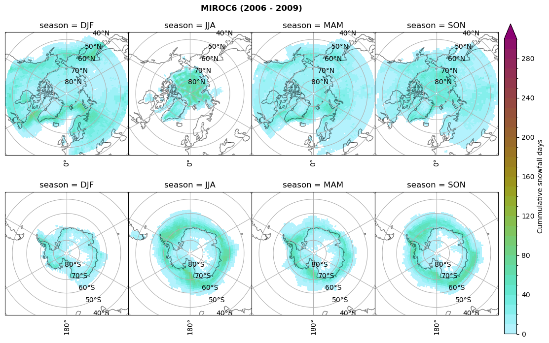
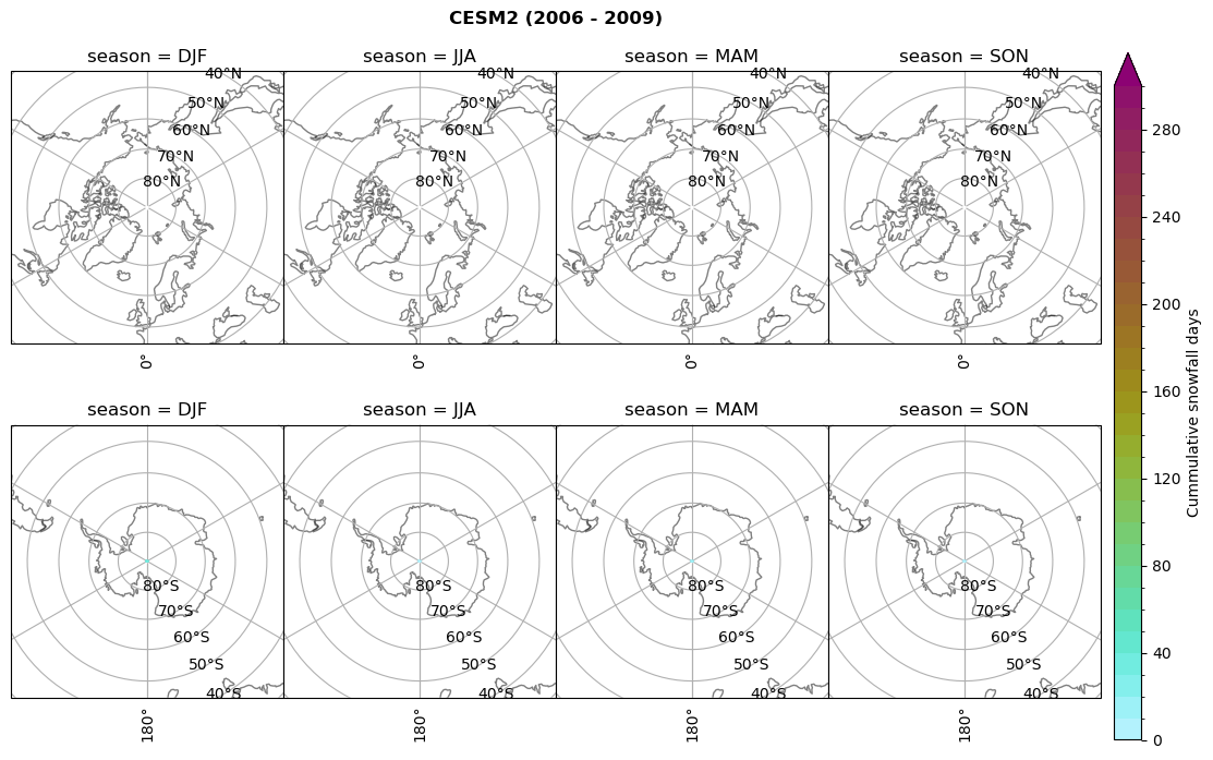
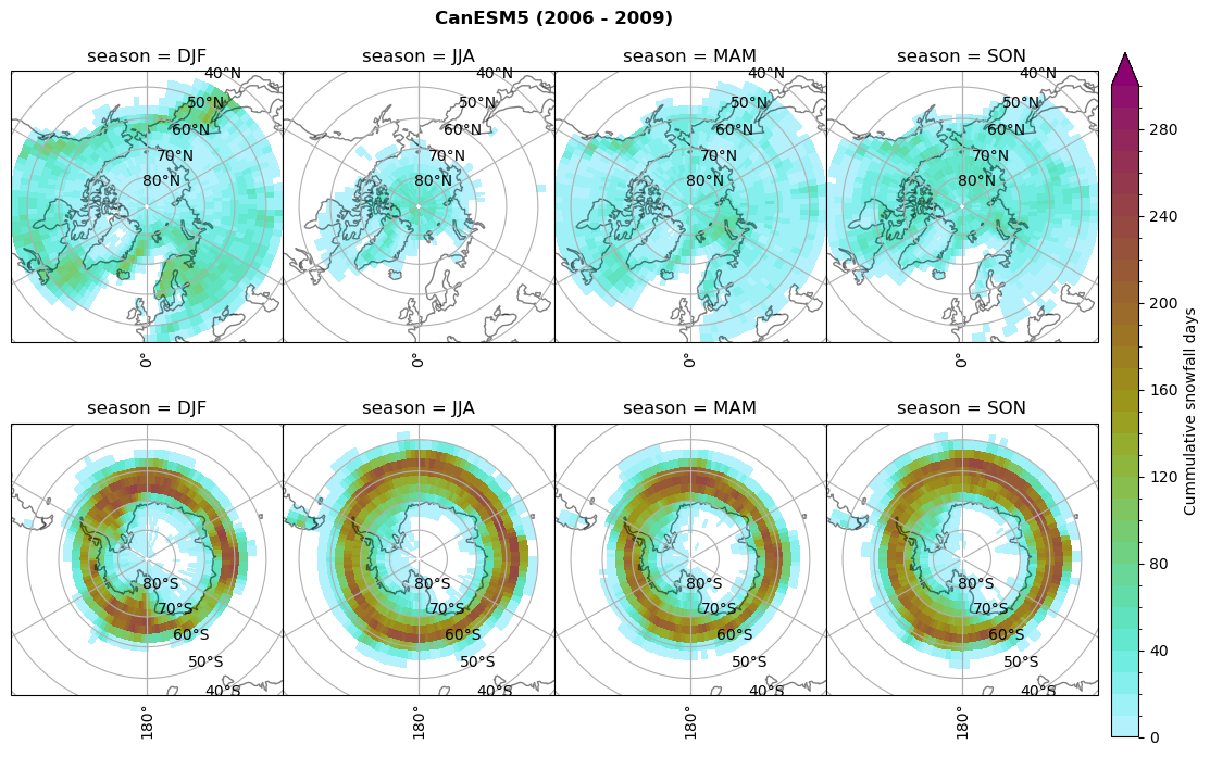
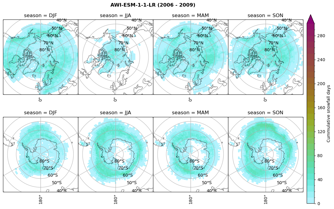
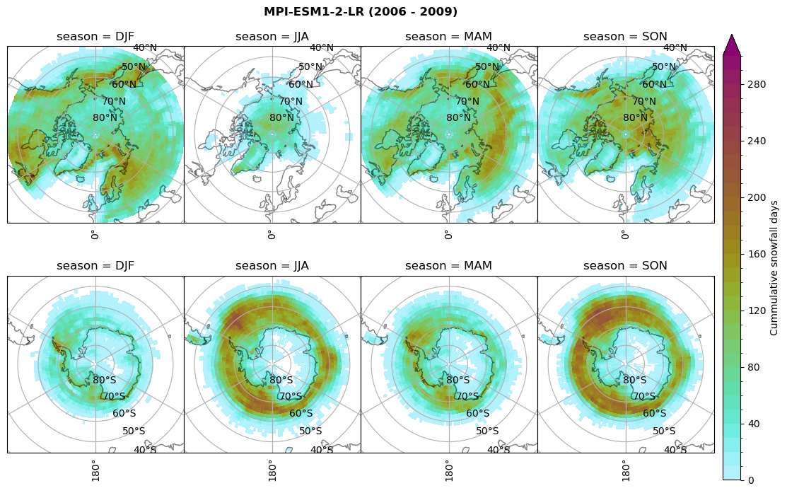
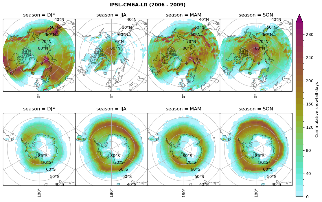
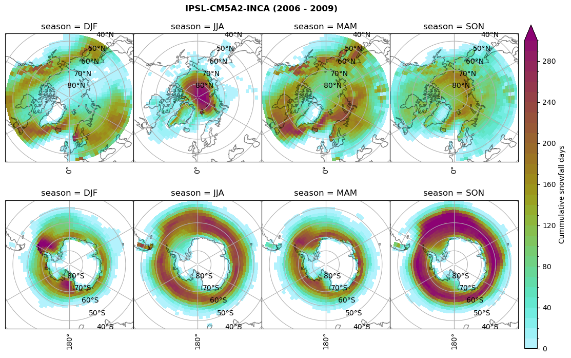
for model in dset_dict.keys():
    # Cummulative snowfall days
    figname = '{}_cum_sf_days_season_mean_{}_{}.png'.format(model,starty, endy)
    plt_seasonal_NH_SH(dset_dict[model]['lcc_count'].where(dset_dict[model]['lcc_count']>0.), levels=np.arange(0,310,10), cbar_label='Cummulative snowfall days', plt_title='{} ({} - {})'.format(model, starty,endy))
    plt.savefig(FIG_DIR + figname, format = 'png', bbox_inches = 'tight', transparent = False)

Calculating bin and bin sizes

https://www.statisticshowto.com/choose-bin-sizes-statistics/

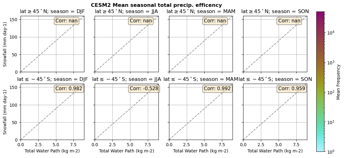
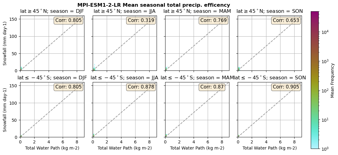
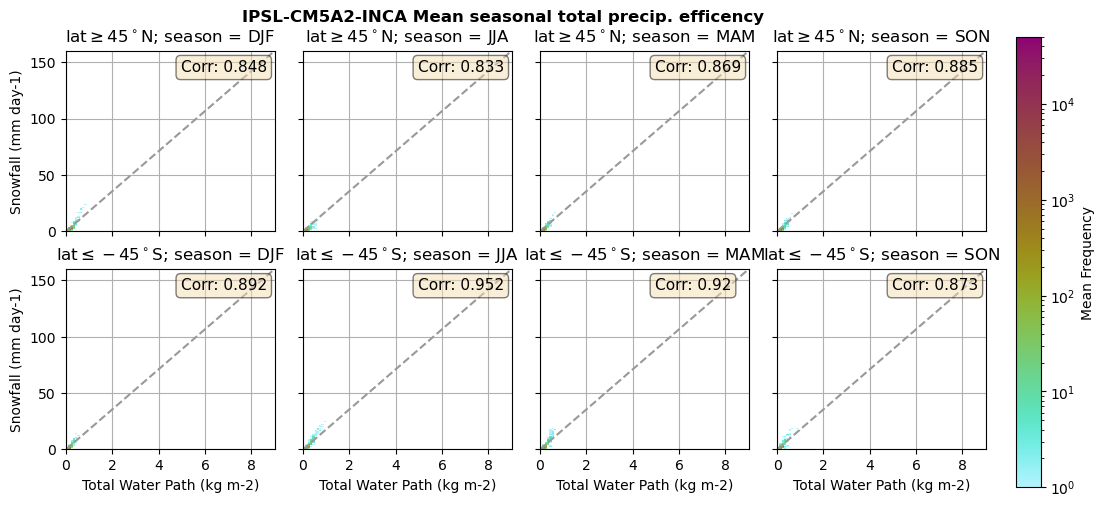
Useful to plot TWP vs. Snowfall (precipitation efficency)

def plt_seasonal_2dhist_wp_sf(x_value, y_value, plt_title, xlabel, ylabel):
    f, axsm = plt.subplots(nrows=2,ncols=4,figsize =[10,5], sharex=True, sharey=True)
    # cmap = cm.batlow
    cmap = cm.hawaii_r
    # levels = np.arange(0.1,65000,5000)
    # norm = BoundaryNorm(levels, ncolors=cmap.N, )
    norm = LogNorm(vmin=1, vmax=50000)



    for ax, season in zip(axsm.flatten()[:4], x_value.season):
        ax.plot([0, 1], [0, 1],ls="--", c=".6", transform=ax.transAxes)
        Z, xedges, yedges = np.histogram2d((x_value.where(x_value['lat'] >=45).sel(season=season).values.flatten()), 
                                        (y_value.where(y_value['lat'] >=45).sel(season=season).values.flatten()), 
                                        bins=[90, 160], 
                                        range=[[0,9],[0, 160]])   

        im = ax.pcolormesh(xedges, yedges, Z.transpose(),cmap=cmap,norm=norm,)
        # cbar = f.colorbar(im, ax=ax,)
        ax.set(title =r'lat$\geq 45^\circ$N; season = {}'.format(season.values))
        ax.grid()
        
        
        _corr = xr.corr(x_value.where(x_value['lat'] >=45).sel(season=season), y_value.where(y_value['lat'] >=45).sel(season=season))
        props = dict(boxstyle='round', facecolor='wheat', alpha=0.5)
        ax.text(0.55, 0.95, 'Corr: {}'.format(np.round(_corr,3).values), transform=ax.transAxes, fontsize=11,
        verticalalignment='top', bbox=props)
        
        

    for ax, season in zip(axsm.flatten()[4:], x_value.season):
        ax.plot([0, 1], [0, 1],ls="--", c=".6", transform=ax.transAxes)
        Z, xedges, yedges = np.histogram2d((x_value.where(x_value['lat'] <=-45).sel(season=season).values.flatten()), 
                                        (y_value.where(y_value['lat'] <=-45).sel(season=season).values.flatten()), 
                                        bins=[90, 160], 
                                        range=[[0,9],[0, 160]])   

        im = ax.pcolormesh(xedges, yedges, Z.transpose(), cmap=cmap,norm=norm,)
        # cbar = f.colorbar(im, ax=ax, )
        ax.set(title =r'lat$\leq-45^\circ$S; season = {}'.format(season.values))
        
        ax.set_xlabel('{} ({})'.format(xlabel,x_value.attrs['units']))
        ax.grid()
        
        _corr = xr.corr(x_value.where(x_value['lat'] <=-45).sel(season=season), y_value.where(y_value['lat'] <=-45).sel(season=season))
        props = dict(boxstyle='round', facecolor='wheat', alpha=0.5)
        ax.text(0.55, 0.95, 'Corr: {}'.format(np.round(_corr,3).values), transform=ax.transAxes, fontsize=11,
        verticalalignment='top', bbox=props)
        
    axsm.flatten()[0].set_ylabel('{} ({})'.format(ylabel, y_value.attrs['units']))
    axsm.flatten()[4].set_ylabel('{} ({})'.format(ylabel, y_value.attrs['units']))


    cbaxes = f.add_axes([1.0125, 0.025, 0.025, 0.9])
    cbar = plt.colorbar(im, cax=cbaxes, shrink=0.5, orientation='vertical', label='Mean Frequency')
    f.suptitle(plt_title, fontweight="bold");
    
    
    
    
    plt.tight_layout(pad=0.5, w_pad=0.5, h_pad=0.5)

for model in dset_dict.keys():
    lwp = dset_dict[model]['lwp_lcc'].groupby('time.season').mean(('time'), keep_attrs=True, skipna=True)
    iwp = dset_dict[model]['iwp_lcc'].groupby('time.season').mean(('time'), keep_attrs=True, skipna=True)
    sf  = dset_dict[model]['sf_lcc'].groupby('time.season').mean(('time'), keep_attrs=True, skipna=True)
    
    # Total water path
    twp = dset_dict[model]['twp_lcc'].groupby('time.season').mean(('time'), keep_attrs=True, skipna=True)
    
    # precip efficency from mixed-phase clouds
    figname = '{}_2dhist_twp_sf_season_mean_{}_{}.png'.format(model, starty, endy)
    plt_seasonal_2dhist_wp_sf(twp, sf, '{} Mean seasonal total precip. efficency'.format(model, ), 'Total Water Path', 'Snowfall')
    plt.savefig(FIG_DIR + figname, format = 'png', bbox_inches = 'tight', transparent = False)

Precipitation efficency - spatial

for model in dset_dict.keys():

    # calculate precipitation efficency
    dset_dict[model]['precip_eff'] = dset_dict[model]['sf_lcc']/dset_dict[model]['twp_lcc']
    
    # calculate days in each season for each year
    sum_day_DJF = dict()
    sum_day_MAM = dict()
    sum_day_JJA = dict()
    sum_day_SON = dict()

    for year in np.unique(dset_dict[model].time.dt.year):
        year=str(year)
        sum_day_DJF[year] = len(dset_dict[model]['precip_eff'].sel(time=year+'-01')) + len(dset_dict[model]['precip_eff'].sel(time=year+'-02')) + len(dset_dict[model]['precip_eff'].sel(time=year+'-12'))
        sum_day_MAM[year] = len(dset_dict[model]['precip_eff'].sel(time=year+'-03')) + len(dset_dict[model]['precip_eff'].sel(time=year+'-04')) + len(dset_dict[model]['precip_eff'].sel(time=year+'-05'))
        sum_day_JJA[year] = len(dset_dict[model]['precip_eff'].sel(time=year+'-06')) + len(dset_dict[model]['precip_eff'].sel(time=year+'-07')) + len(dset_dict[model]['precip_eff'].sel(time=year+'-08'))
        sum_day_SON[year] = len(dset_dict[model]['precip_eff'].sel(time=year+'-09')) + len(dset_dict[model]['precip_eff'].sel(time=year+'-10')) + len(dset_dict[model]['precip_eff'].sel(time=year+'-11'))

    days_DJF = sum(sum_day_DJF.values())
    days_MAM = sum(sum_day_MAM.values())
    days_JJA = sum(sum_day_JJA.values())
    days_SON = sum(sum_day_SON.values())

    # calculate sum of monthly precip eff
    precip_eff_mon = dset_dict[model]['precip_eff'].groupby('time.month').sum('time',skipna=True)

    # calculate sum of each season precipitation eff
    precip_eff = dict()
    precip_eff['DJF'] = (precip_eff_mon.sel(month=1) + precip_eff_mon.sel(month=2) + precip_eff_mon.sel(month=12))/days_DJF
    precip_eff['MAM'] = (precip_eff_mon.sel(month=3) + precip_eff_mon.sel(month=4) + precip_eff_mon.sel(month=5))/days_MAM
    precip_eff['JJA'] = (precip_eff_mon.sel(month=6) + precip_eff_mon.sel(month=7) + precip_eff_mon.sel(month=8))/days_JJA
    precip_eff['SON'] = (precip_eff_mon.sel(month=9) + precip_eff_mon.sel(month=10) + precip_eff_mon.sel(month=11))/days_SON

    _da = list(precip_eff.values())
    _coord = list(precip_eff.keys())
    # _da = list(pe.values())
    # _coord = list(pe.keys())    
    dset_dict[model]['precip_eff_seas'] = xr.concat(objs=_da, dim=_coord, coords='all').rename({'concat_dim':'season'})
    
    # Plot precipitation efficency
    plt_seasonal_NH_SH(dset_dict[model]['precip_eff_seas'], np.arange(0., 15.5,.5), 'relative snowfall eff.', '{} ({} - {})'.format(model,starty,endy))

    # save precip efficency from mixed-phase clouds figure
    figname = '{}_sf_twp_season_mean_{}_{}.png'.format(model, starty, endy)
    plt.savefig(FIG_DIR + figname, format = 'png', bbox_inches = 'tight', transparent = False)
        
        

Relative frequency

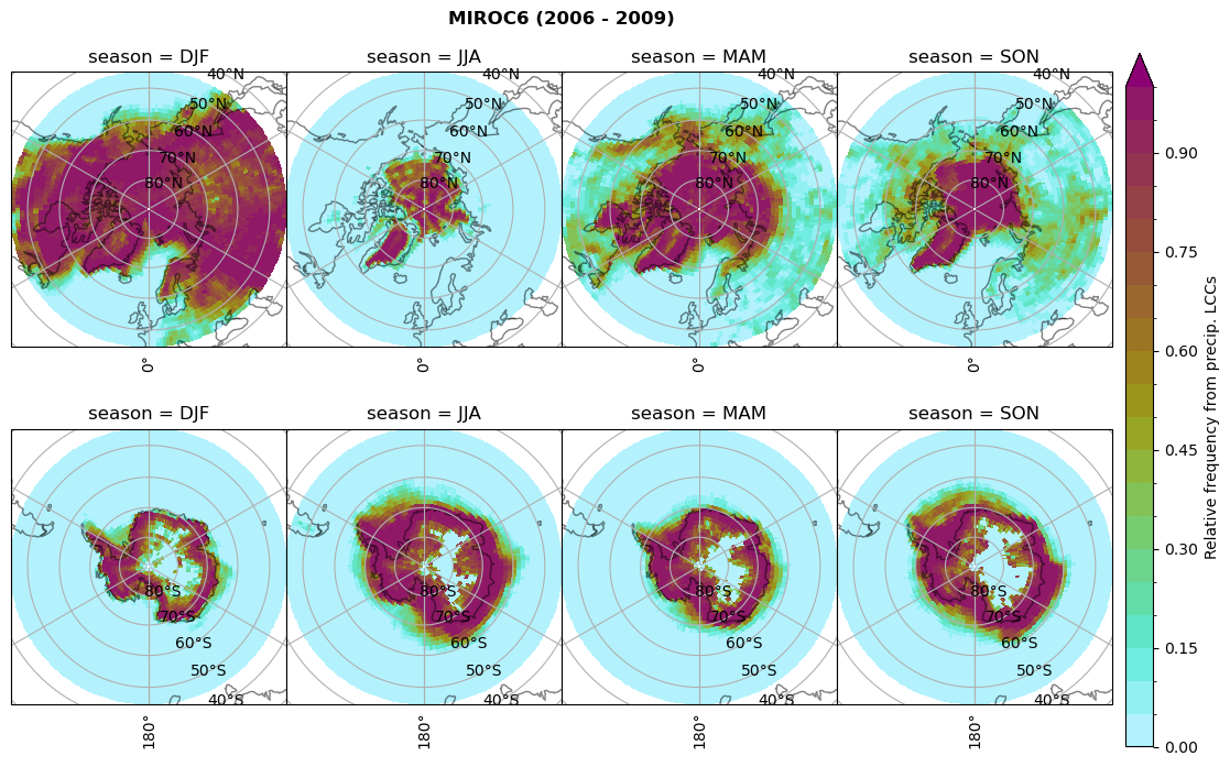
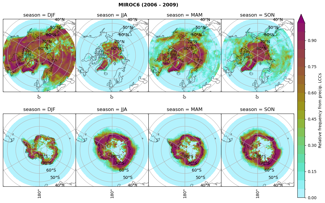
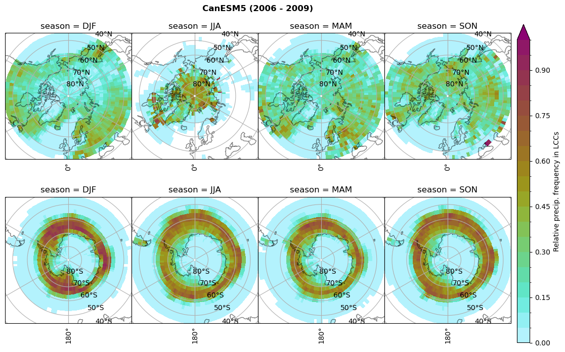
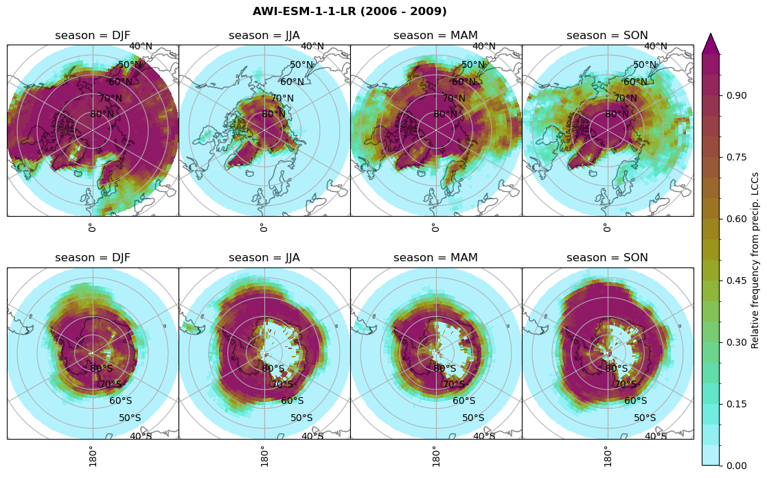
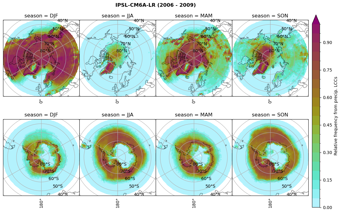
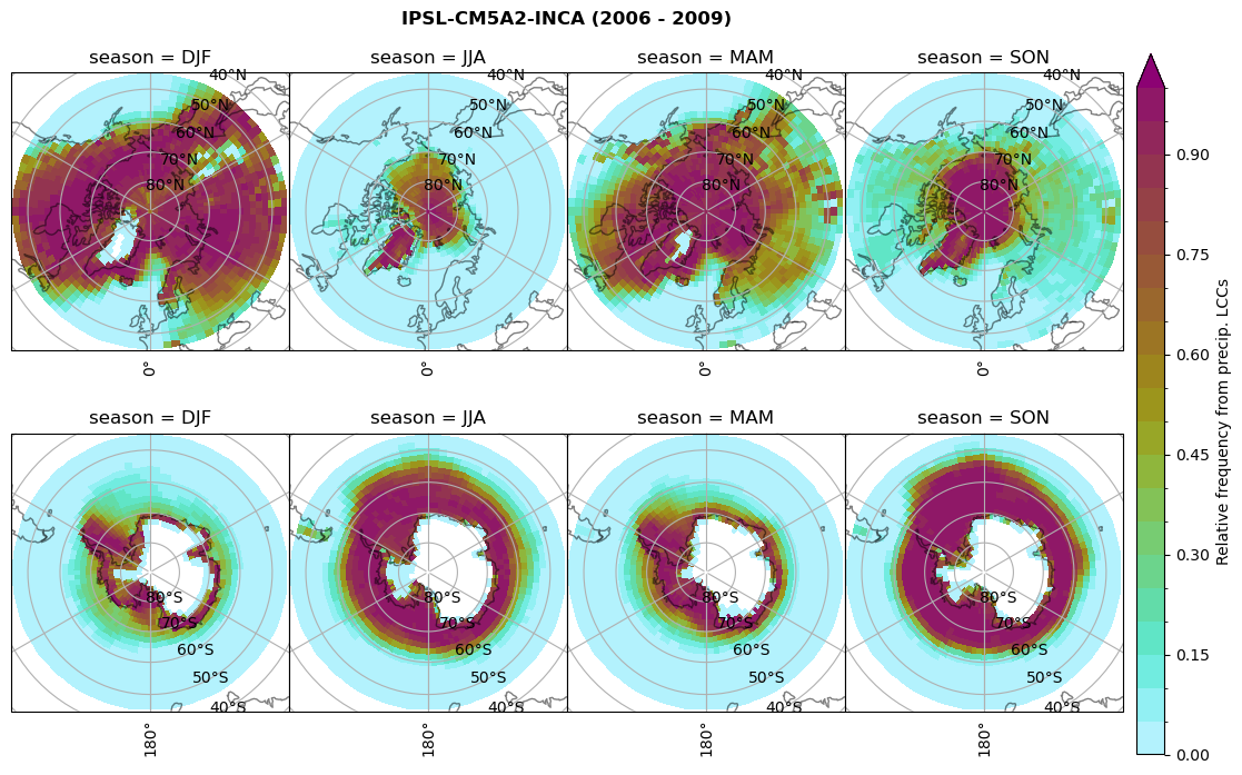
\[RF = \frac{f}{n} = \frac{\text{number of times the data occurred in an observation}}{\text{total frequency}}\]

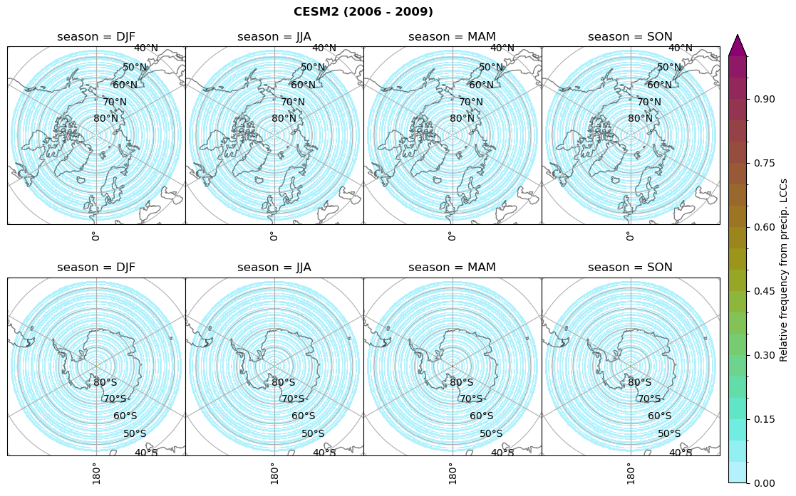
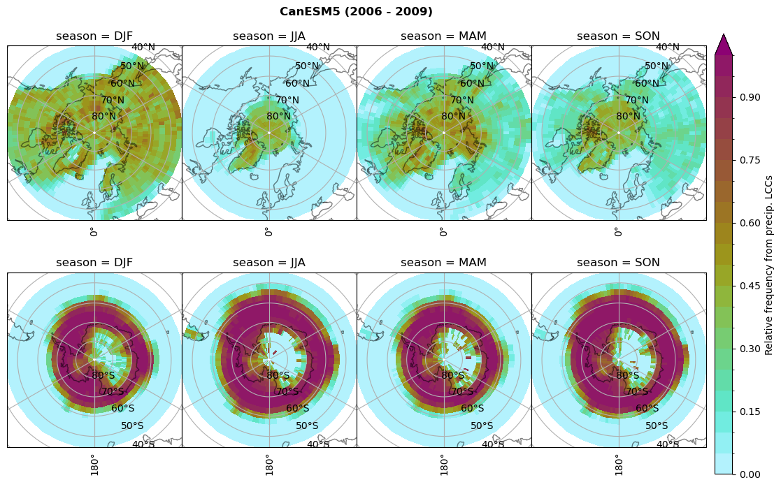
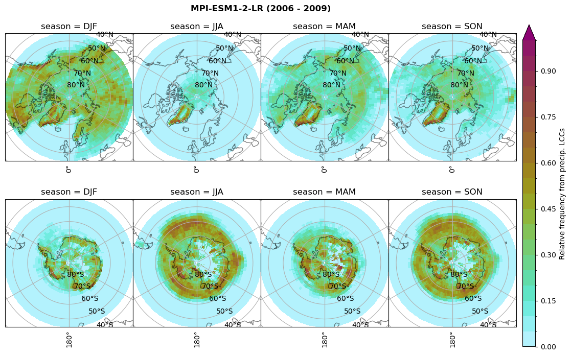
for model in dset_dict.keys():
    # frequency without snow requirement
    n = dset_dict[model]['lwp'].groupby('time.season').sum('time',skipna=True)
    f= dset_dict[model]['lwp_lcc2'].groupby('time.season').sum('time',skipna=True)
    dset_dict[model]['rf_lcc_wo_snow'] = f/n
    plt_seasonal_NH_SH(dset_dict[model]['rf_lcc_wo_snow'], np.arange(0,1.05,0.05), 'Relative frequency from precip. LCCs', '{} ({} - {})'.format(model,starty,endy))
    # save frequency from LCCs
    figname = '{}_rf_lcc_wo_snow_season_{}_{}.png'.format(model, starty, endy)
    plt.savefig(FIG_DIR + figname, format = 'png', bbox_inches = 'tight', transparent = False)
    
    
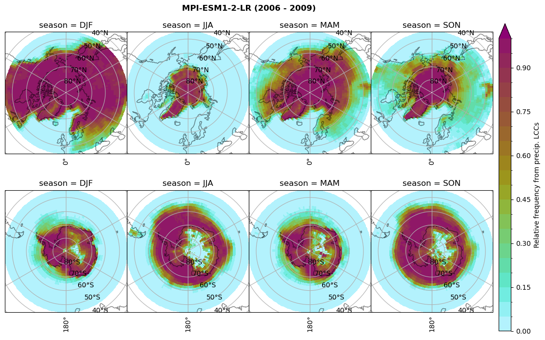
    # frequency with snow from lccs
    n = dset_dict[model]['lwp'].groupby('time.season').sum('time',skipna=True)
    f= dset_dict[model]['lwp_lcc'].groupby('time.season').sum('time',skipna=True)
    dset_dict[model]['rf_lcc_w_snow'] = f/n
    plt_seasonal_NH_SH(dset_dict[model]['rf_lcc_w_snow'], np.arange(0,1.05,0.05), 'Relative frequency from precip. LCCs', '{} ({} - {})'.format(model,starty,endy))
    # save frequency from LCCs
    figname = '{}_rf_lcc_w_snow_season_{}_{}.png'.format(model,starty, endy)
    plt.savefig(FIG_DIR + figname, format = 'png', bbox_inches = 'tight', transparent = False)
    
    
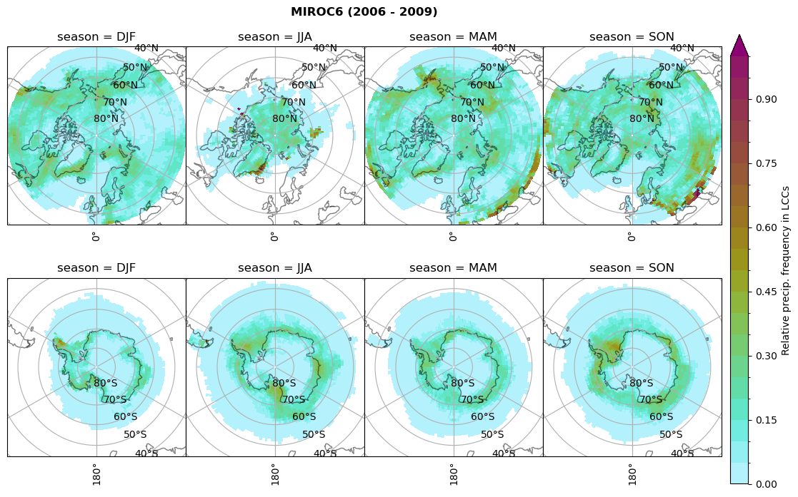
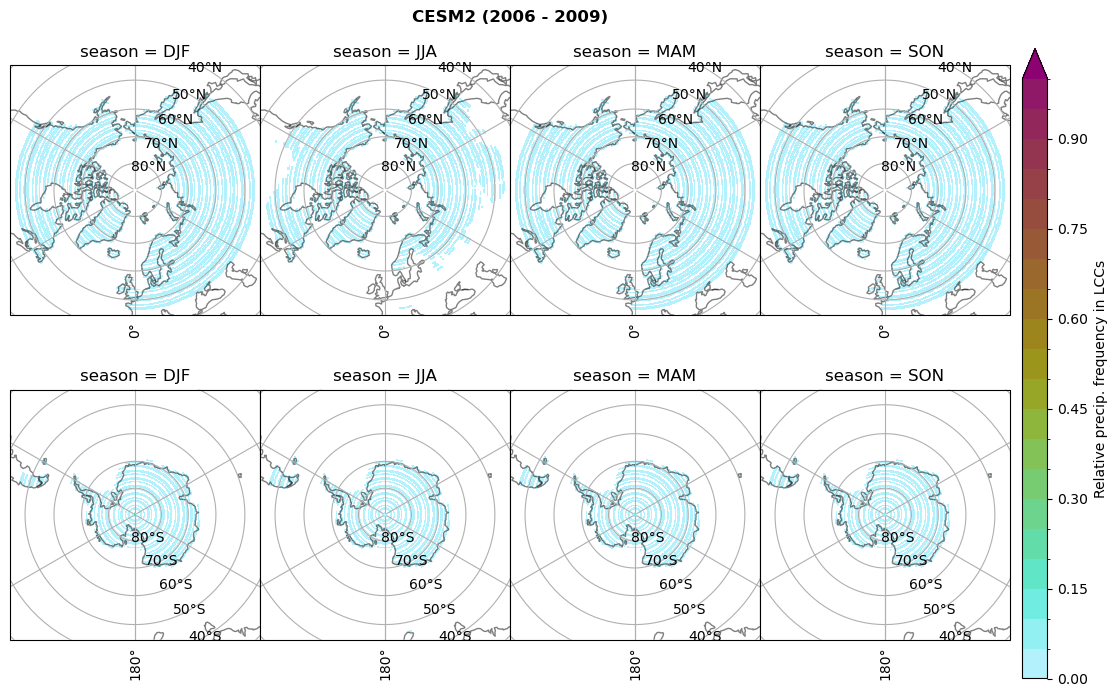
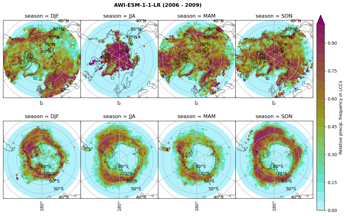
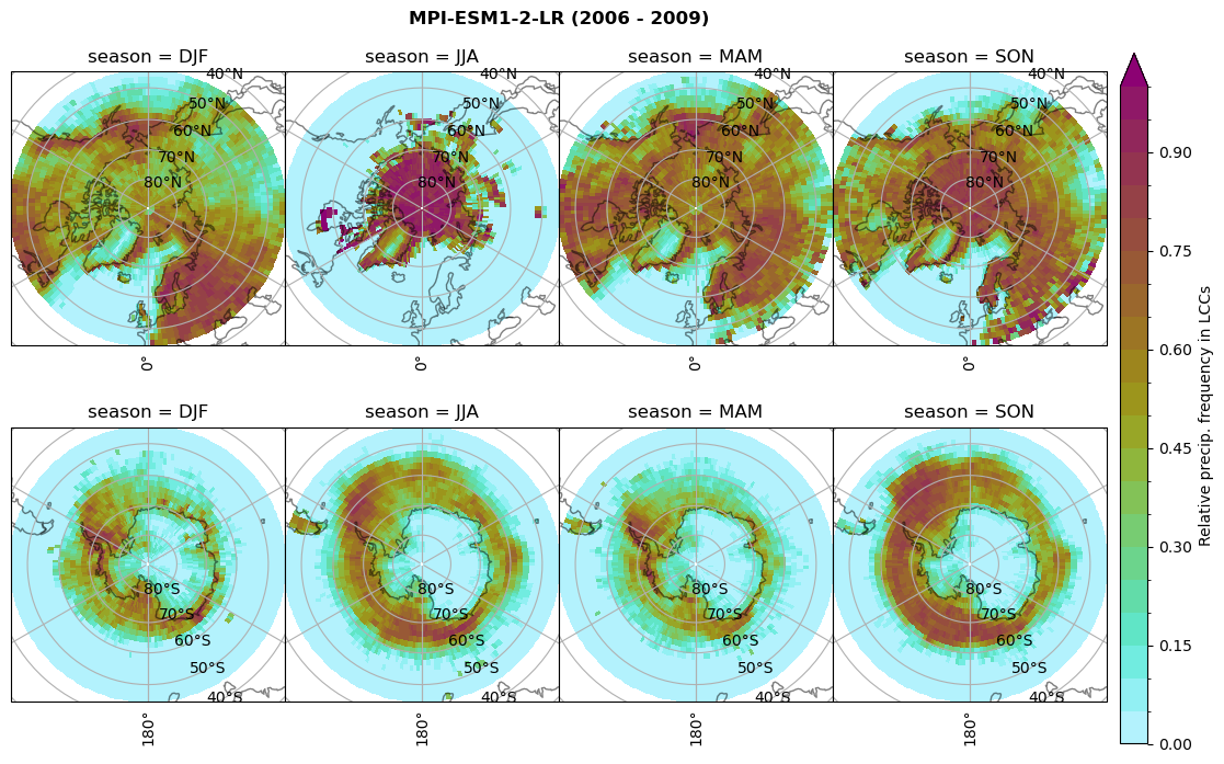
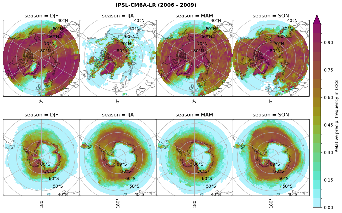
    n = dset_dict[model]['prsn'].groupby('time.season').sum('time',skipna=True)
    f= dset_dict[model]['sf_lcc'].groupby('time.season').sum('time',skipna=True)
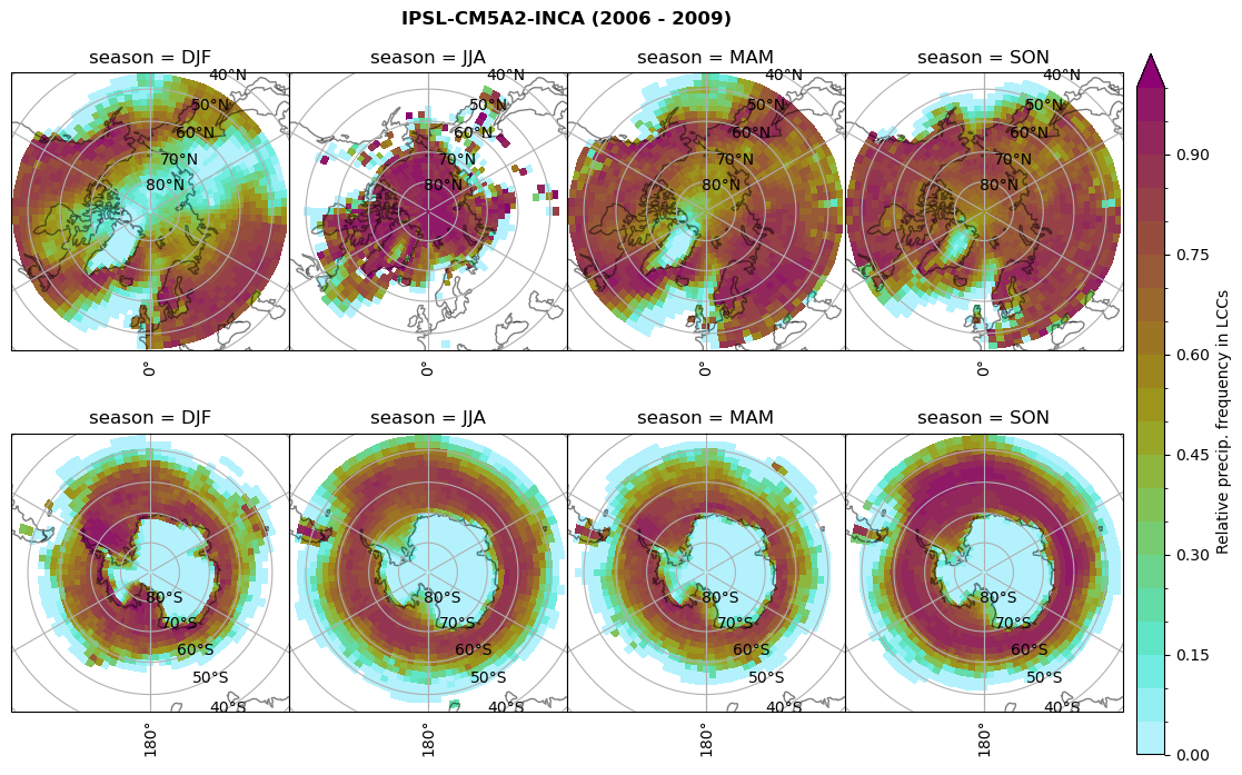
    dset_dict[model]['rf_sf_lcc'] = f/n
    plt_seasonal_NH_SH(dset_dict[model]['rf_sf_lcc'], np.arange(0,1.05,0.05), 'Relative precip. frequency in LCCs', '{} ({} - {})'.format(model,starty,endy))
    # save frequency from LCCs
    figname = '{}_rf_sf_lcc_season_{}_{}.png'.format(model,starty, endy)
    plt.savefig(FIG_DIR + figname, format = 'png', bbox_inches = 'tight', transparent = False)
    

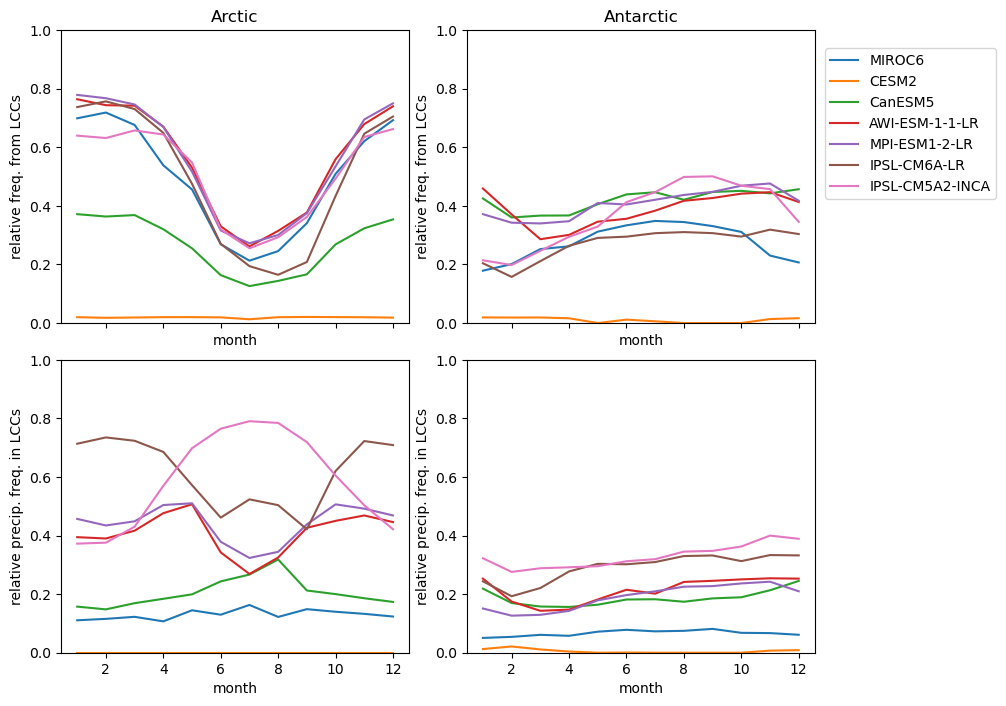
Plot annual cycle of LCC frequency, precipitaiton frequency in LCCs, relative snowfall efficeny

lcc_wo_snow_NH = {}
lcc_wo_snow_SH = {}

sf_lcc_NH = {}
sf_lcc_SH = {}
for model in dset_dict.keys():
    n = dset_dict[model]['lwp'].groupby('time.month').sum('time',skipna=True)
    f = dset_dict[model]['lwp_lcc2'].groupby('time.month').sum('time',skipna=True)
    rf_lcc_wo_snow = f/n

    lcc_wo_snow_NH[model] = ((rf_lcc_wo_snow.sel(lat=slice(45,90))).mean(('lon','lat'),skipna=True))
    lcc_wo_snow_SH[model] = ((rf_lcc_wo_snow.sel(lat=slice(-90,-45))).mean(('lon','lat'),skipna=True))
    
    
    n = dset_dict[model]['prsn'].groupby('time.month').sum('time',skipna=True)
    f= dset_dict[model]['sf_lcc'].groupby('time.month').sum('time',skipna=True)
    rf_sf_lcc = f/n
    
    sf_lcc_NH[model] = ((rf_sf_lcc.sel(lat=slice(45,90))).mean(('lon','lat'),skipna=True))
    sf_lcc_SH[model] = ((rf_sf_lcc.sel(lat=slice(-90,-45))).mean(('lon','lat'),skipna=True))
    
    try:
        lcc_wo_snow_NH[model] = lcc_wo_snow_NH[model].drop('height')
        lcc_wo_snow_SH[model] = lcc_wo_snow_SH[model].drop('height')
        
        sf_lcc_NH[model] = sf_lcc_NH[model].drop('height')
        sf_lcc_SH[model] = sf_lcc_SH[model].drop('height')
    except ValueError:
        continue

ratios = xr.Dataset()
_da = list(lcc_wo_snow_NH.values())
_coord = list(lcc_wo_snow_NH.keys())

ratios['lcc_wo_snow_NH'] = xr.concat(objs=_da, dim=_coord, coords='all').rename({'concat_dim':'model'})
    
_da = list(lcc_wo_snow_SH.values())
_coord = list(lcc_wo_snow_SH.keys())

ratios['lcc_wo_snow_SH'] = xr.concat(objs=_da, dim=_coord, coords='all').rename({'concat_dim':'model'})
_da = list(sf_lcc_NH.values())
_coord = list(sf_lcc_NH.keys())

ratios['sf_lcc_NH'] = xr.concat(objs=_da, dim=_coord, coords='all').rename({'concat_dim':'model'})
_da = list(sf_lcc_SH.values())
_coord = list(sf_lcc_SH.keys())

ratios['sf_lcc_SH'] = xr.concat(objs=_da, dim=_coord, coords='all').rename({'concat_dim':'model'})

ds_era0 = xr.open_dataset('/scratch/franzihe/output/ERA5/daily_means/model_grid/ERA5_daily_mean_ERA5_200701_201012.nc')

---------------------------------------------------------------------------
AttributeError                            Traceback (most recent call last)
Cell In [71], line 1
----> 1 ds_era0 = xr.opendataset('/scratch/franzihe/output/ERA5/daily_means/model_grid/ERA5_daily_mean_ERA5_200701_201012.nc')

AttributeError: module 'xarray' has no attribute 'opendataset'

f, axsm = plt.subplots(nrows=2,ncols=2,figsize =[10,7], sharex=True)

ax = axsm.flatten()
ratios['lcc_wo_snow_NH'].plot.line(ax=ax[0], x='month', hue='model', add_legend=False, ylim=[0,1])
ratios['lcc_wo_snow_SH'].plot.line(ax=ax[1], x='month', hue='model', add_legend=False, ylim=[0,1])
ratios['sf_lcc_NH'].plot.line(ax=ax[2], x='month', hue='model', add_legend=False, ylim=[0,1])
ratios['sf_lcc_SH'].plot.line(ax=ax[3], x='month', hue='model', add_legend=False, ylim=[0,1])

ax[0].set_ylabel('relative freq. from LCCs')
ax[0].set(title ='Arctic')
ax[1].set_ylabel('relative freq. from LCCs')
ax[1].set(title ='Antarctic')

ax[2].set_ylabel('relative precip. freq. in LCCs')
ax[3].set_ylabel('relative precip. freq. in LCCs')


ax[1].legend(list(ratios['model'].values), bbox_to_anchor=(1.01, .4, -1., .102), loc='lower left', ncol = 1)
plt.tight_layout(pad=0.5, w_pad=0.5, h_pad=0.5)

Load ERA5 data in model resolutions

ds_era = dict()
for model in dset_dict.keys():
    ds_era[model] = xr.open_mfdataset(glob('{}/ERA5/daily_means/model_grid/*{}*.nc'.format(OUTPUT_DATA_DIR,model)))
    
    # remove leap day from dataset
    ds_era[model] = ds_era[model].sel(time=~((ds_era[model].time.dt.month == 2) & (ds_era[model].time.dt.day == 29)))

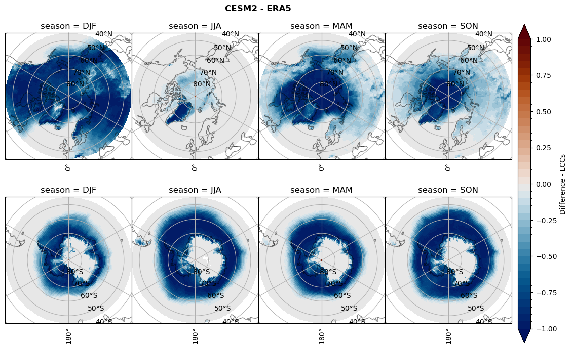
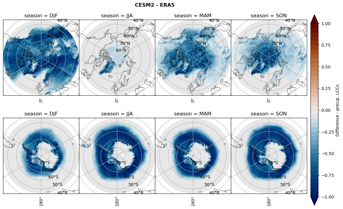
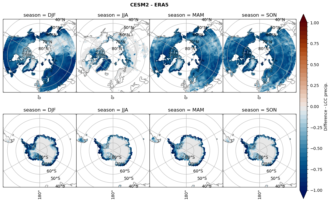
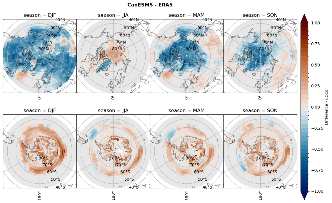
Differences Model - ERA5

def plt_seasonal_diff(variable, levels, cbar_label, plt_title):
    f, axsm = plt.subplots(nrows=2,ncols=4,figsize =[10,7], subplot_kw={'projection': ccrs.NorthPolarStereo(central_longitude=0.0,globe=None)})

    coast = cy.feature.NaturalEarthFeature(category='physical', scale='110m',
                            facecolor='none', name='coastline')
    
    for ax, season in zip(axsm.flatten()[:4], variable.season):
        # ax.add_feature(cy.feature.COASTLINE, alpha=0.5)
        ax.add_feature(coast,alpha=0.5)
        ax.set_extent([-180, 180, 90, 45], ccrs.PlateCarree())
        gl = ax.gridlines(draw_labels=True)
        gl.top_labels   = False
        gl.right_labels = False
        variable.sel(season=season, lat=slice(45,90)).plot(ax=ax, transform=ccrs.PlateCarree(), extend='both', add_colorbar=False,
                            cmap=cm.vik, levels=levels)
        ax.set(title ='season = {}'.format(season.values))

    for ax, i, season in zip(axsm.flatten()[4:], np.arange(5,9), variable.season):
        ax.remove()
        ax = f.add_subplot(2,4,i, projection=ccrs.SouthPolarStereo(central_longitude=0.0, globe=None))
        # ax.add_feature(cy.feature.COASTLINE, alpha=0.5)
        ax.add_feature(coast,alpha=0.5)
        ax.set_extent([-180, 180, -90, -45], ccrs.PlateCarree())
        gl = ax.gridlines(draw_labels=True)
        gl.top_labels   = False
        gl.right_labels = False
        cf = variable.sel(season=season, lat=slice(-90,-45)).plot(ax=ax, transform=ccrs.PlateCarree(), extend='both', add_colorbar=False,
                            cmap=cm.vik,levels=levels)
        ax.set(title ='season = {}'.format(season.values))

    cbaxes = f.add_axes([1.0125, 0.025, 0.025, 0.9])
    cbar = plt.colorbar(cf, cax=cbaxes, shrink=0.5,extend='both', orientation='vertical', label=cbar_label)
    f.suptitle(plt_title, fontweight="bold");
    plt.tight_layout(pad=0., w_pad=0., h_pad=0.)

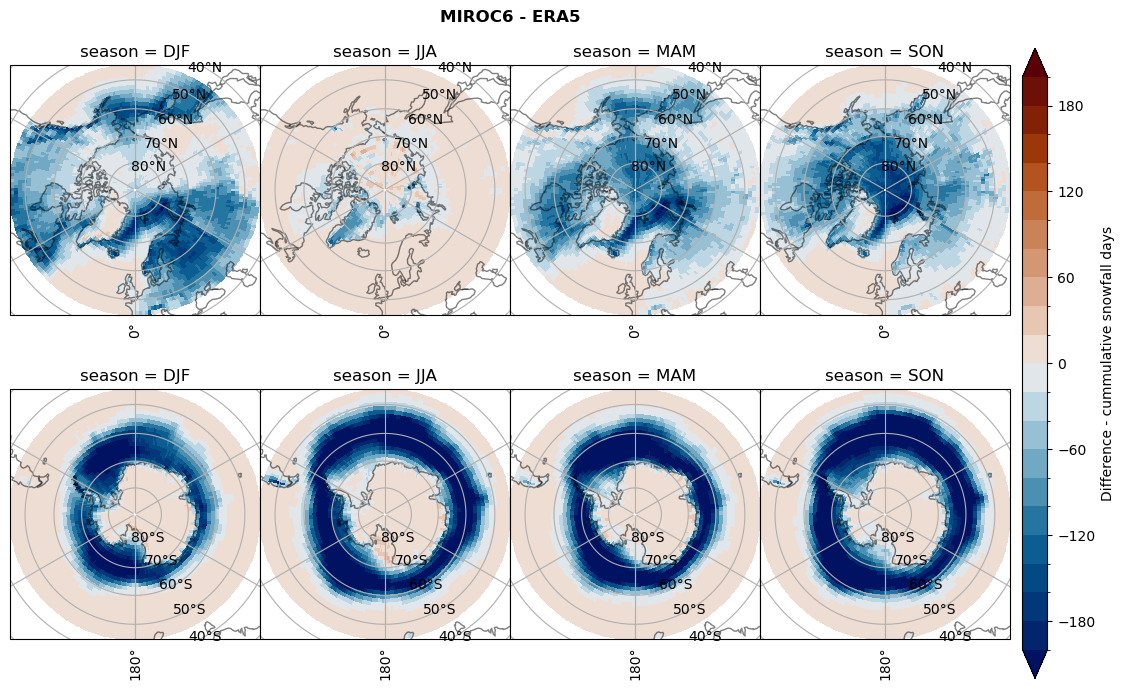
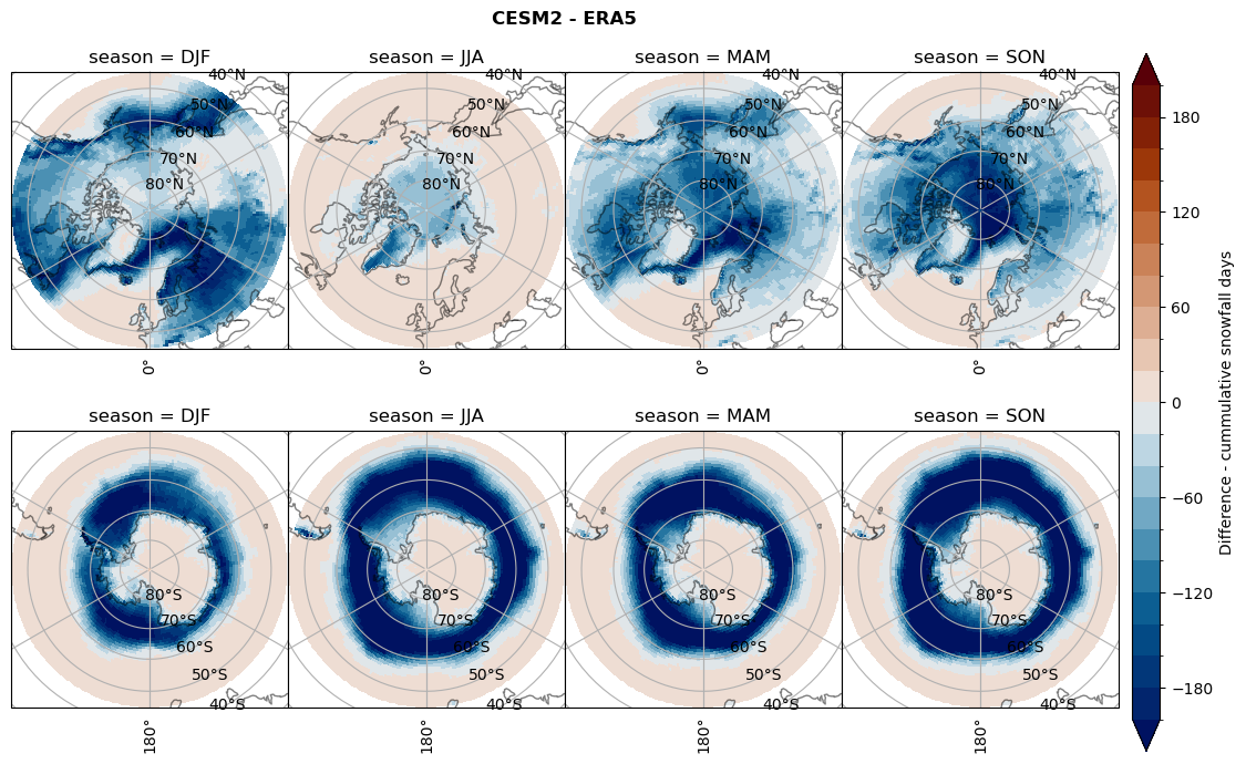
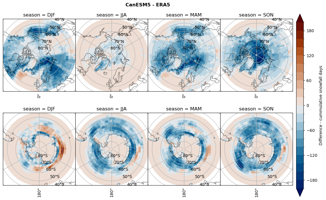
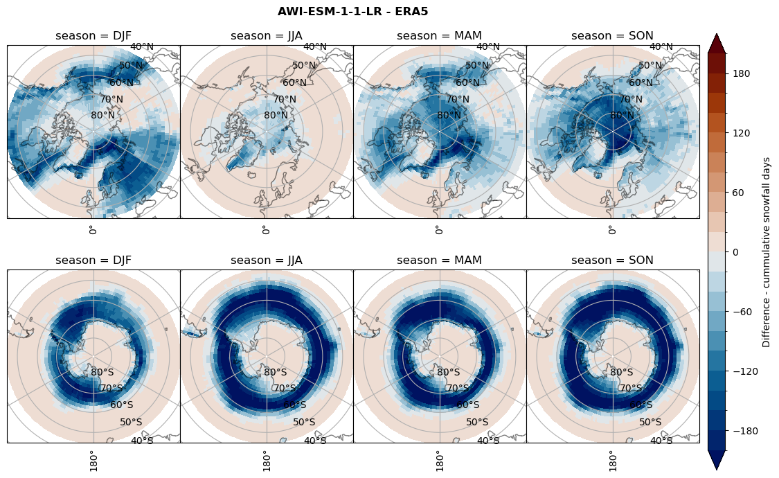
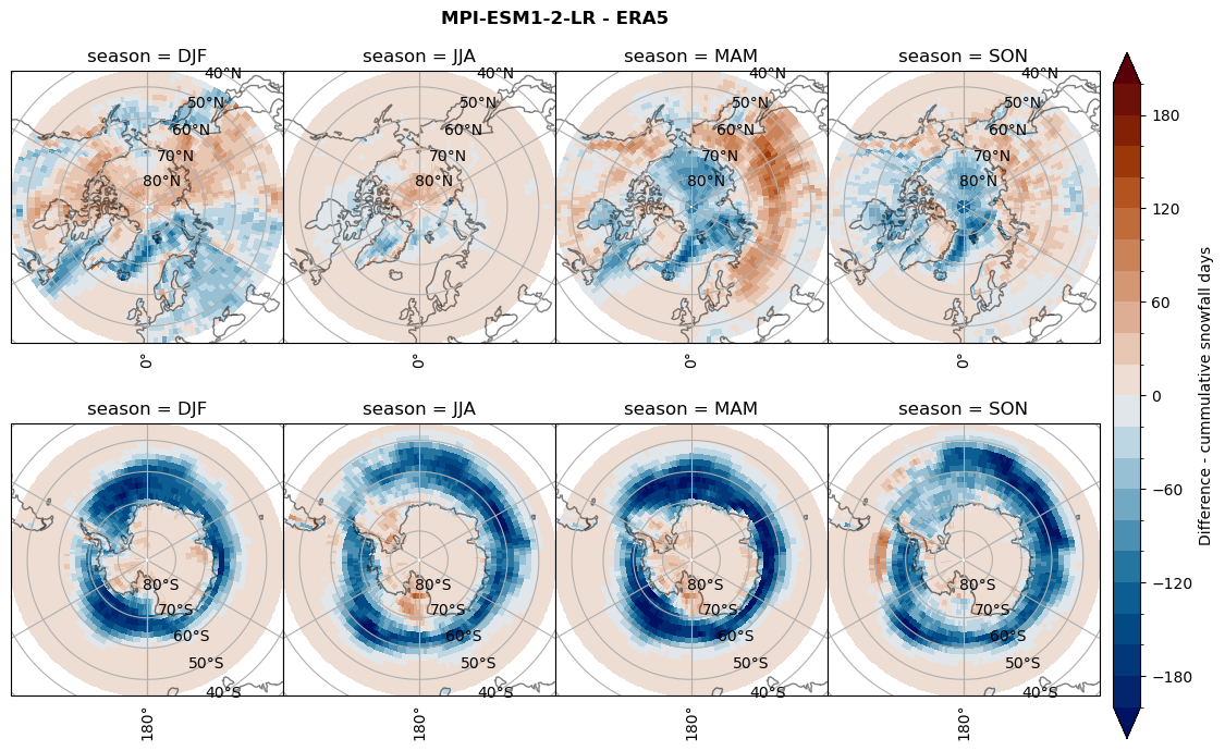
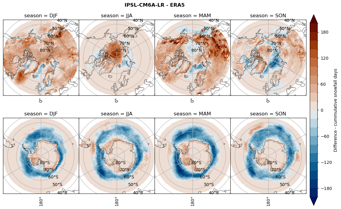
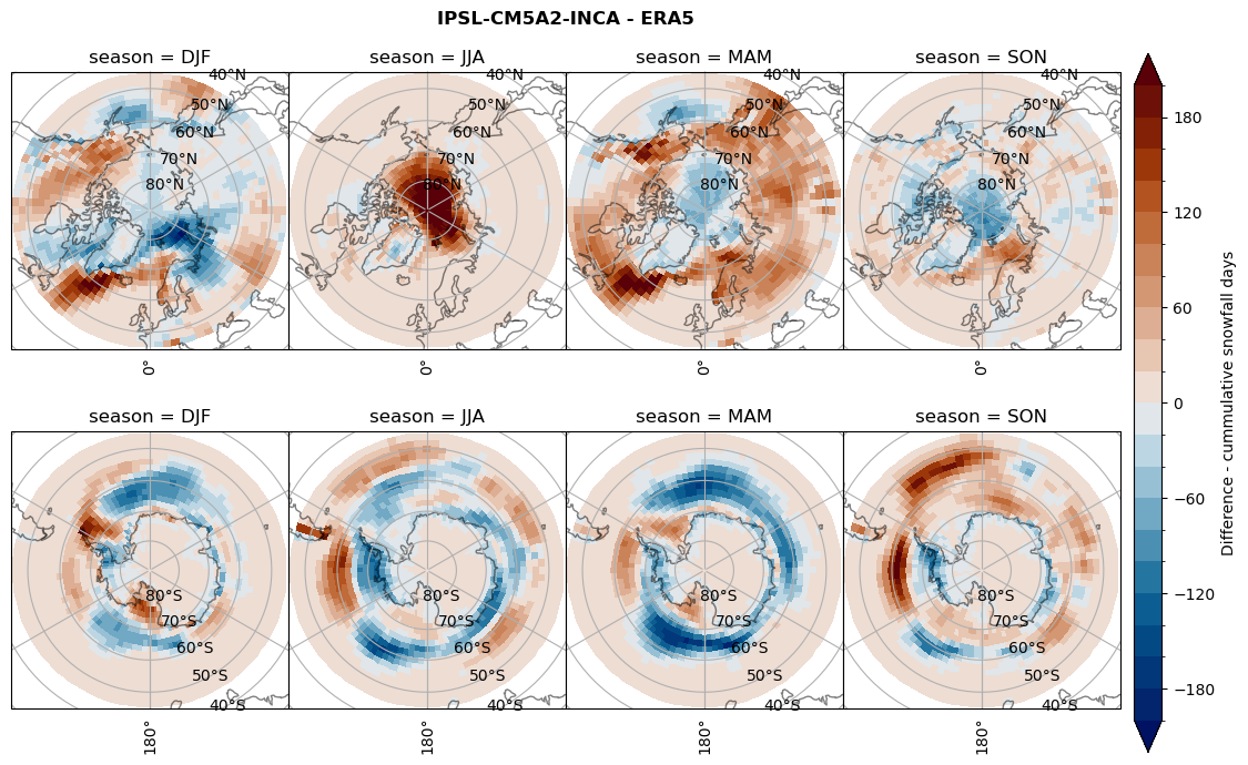
Difference Cummulative snowfall days

for model in dset_dict.keys():
    variable = dset_dict[model]['lcc_count'] - ds_era[model]['lcc_count']
    plt_title = '{} - ERA5'.format(model)
    levels = np.arange(-200, 220, 20)
    cbar_label = 'Difference - cummulative snowfall days'
    
    plt_seasonal_diff(variable, levels, cbar_label, plt_title)
    
    figname = '{}_diff_cum_sf_days_season_mean_{}_{}.png'.format(model,starty, endy)
    plt.savefig(FIG_DIR + figname, format = 'png', bbox_inches = 'tight', transparent = False)

    

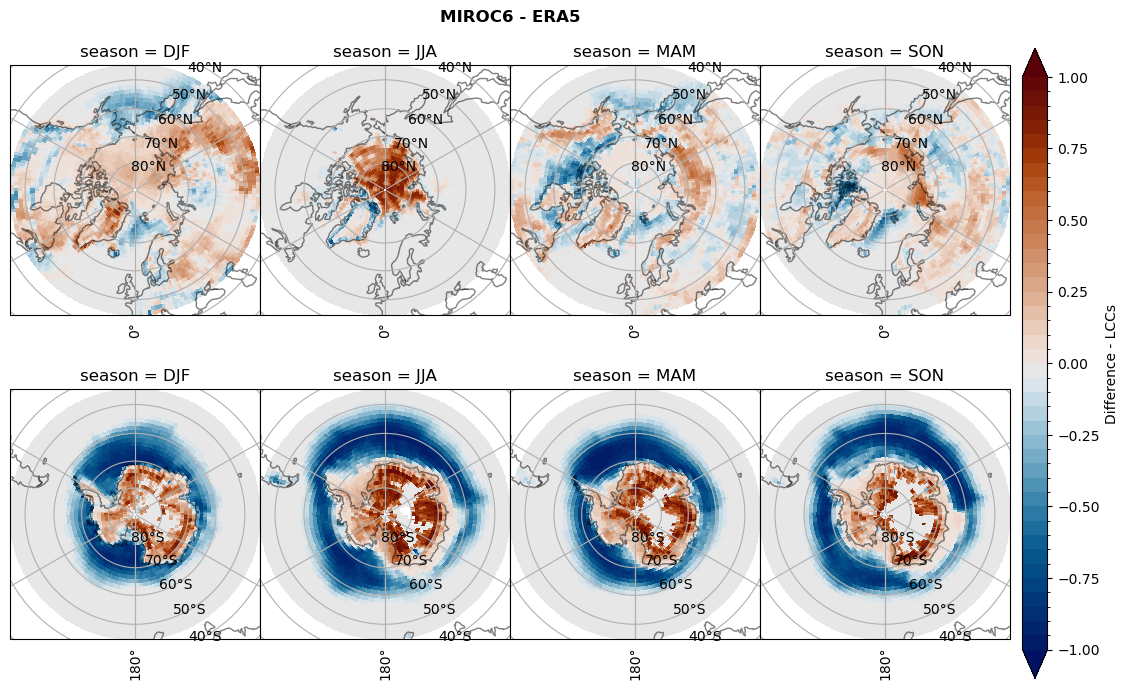
Difference Frequencys

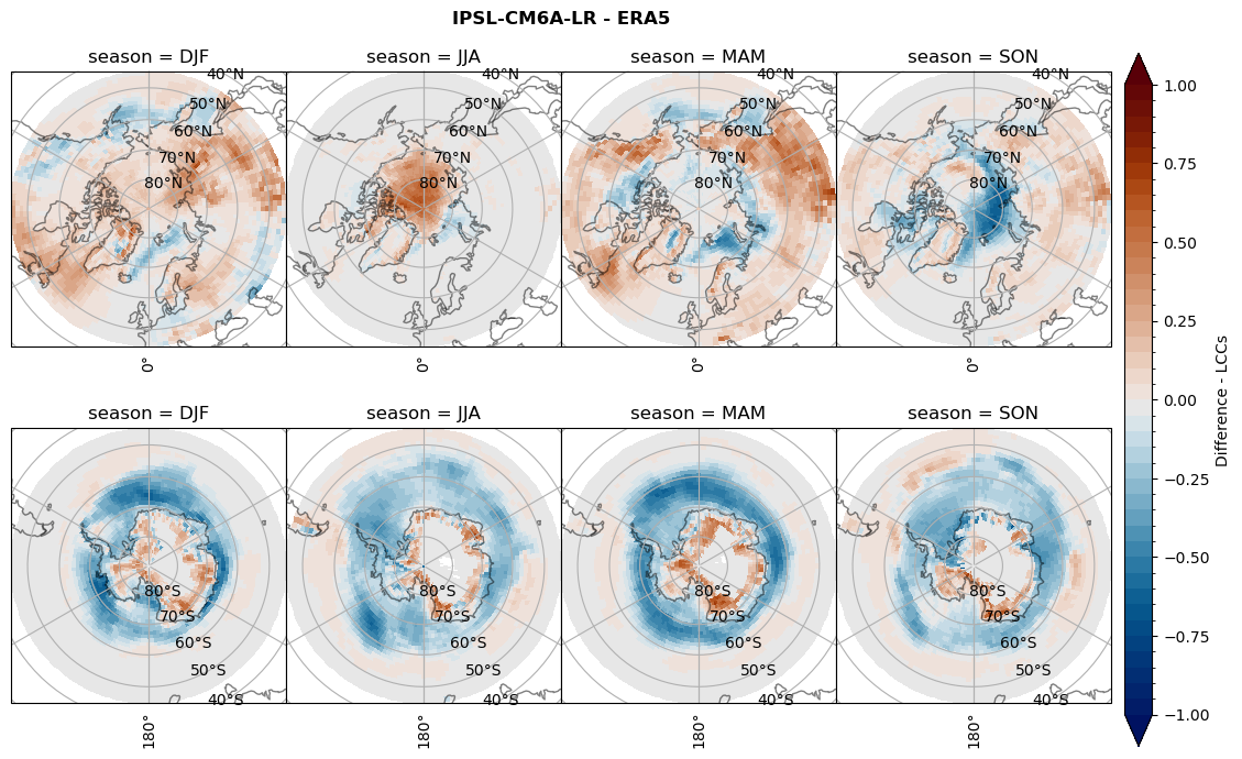
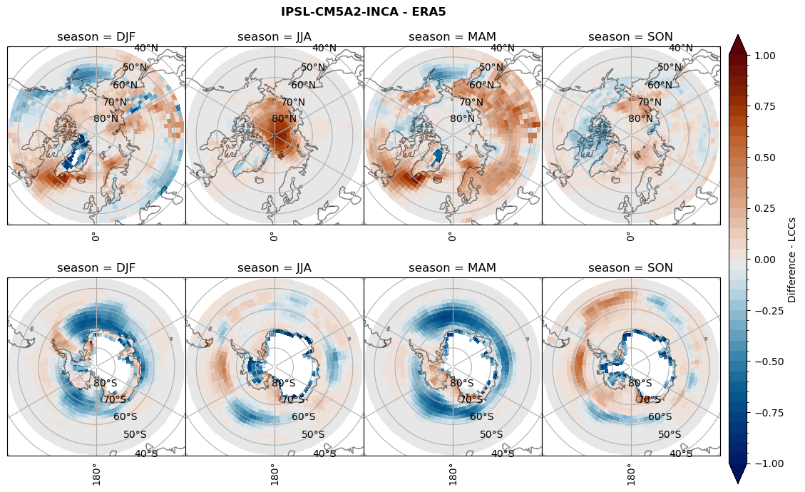
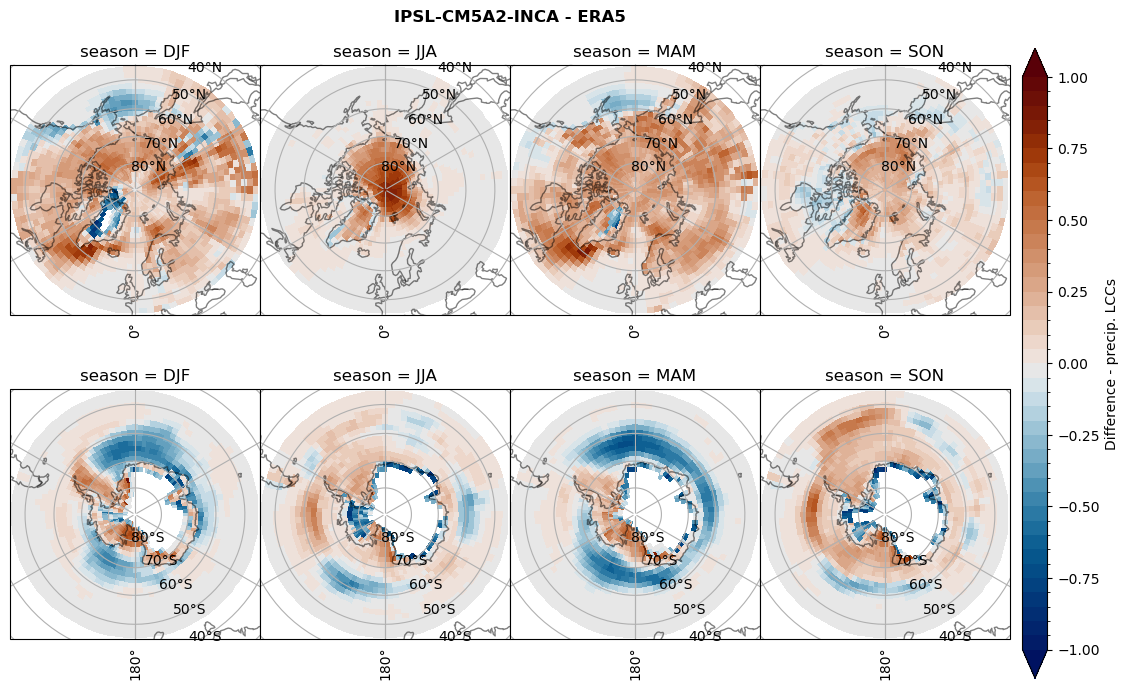
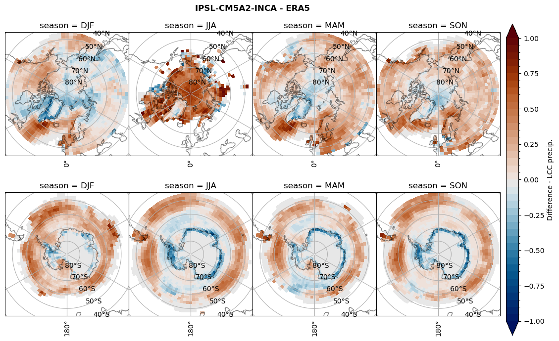
for model in dset_dict.keys():
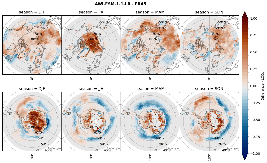
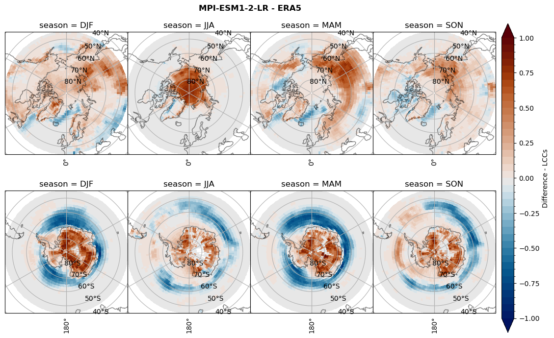
    # Difference relative frequency lccs without snow requirement
    rf_lcc_wo_snow = dset_dict[model]['rf_lcc_wo_snow'] - ds_era[model]['rf_lcc_wo_snow']
    plt_title = '{} - ERA5'.format(model)
    levels = np.arange(-1.0, 1.05, 0.05)
    cbar_label = 'Difference - LCCs'
    plt_seasonal_diff(rf_lcc_wo_snow, levels,cbar_label, plt_title)
    figname = '{}_diff_rf_lcc_wo_snow_season_{}_{}.png'.format(model,starty, endy)
    plt.savefig(FIG_DIR + figname, format = 'png', bbox_inches = 'tight', transparent = False)
    
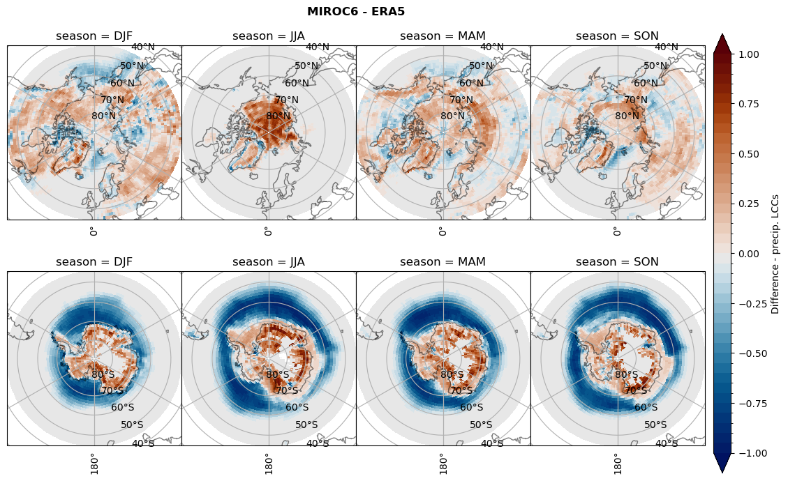
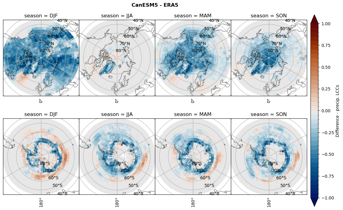
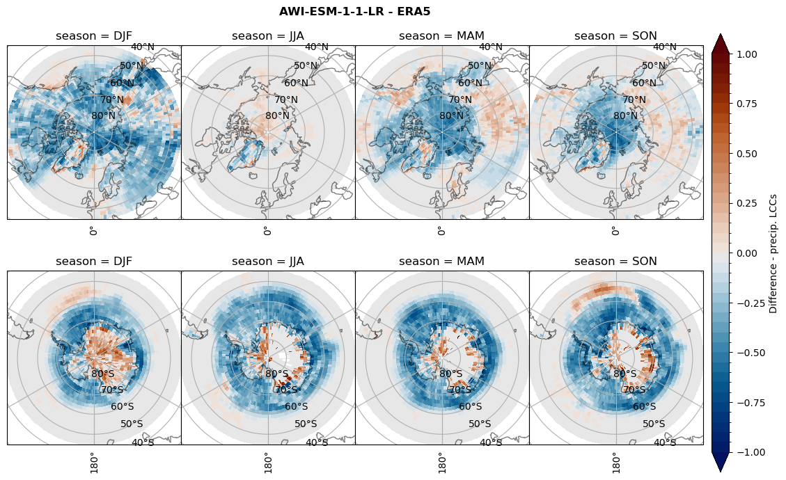
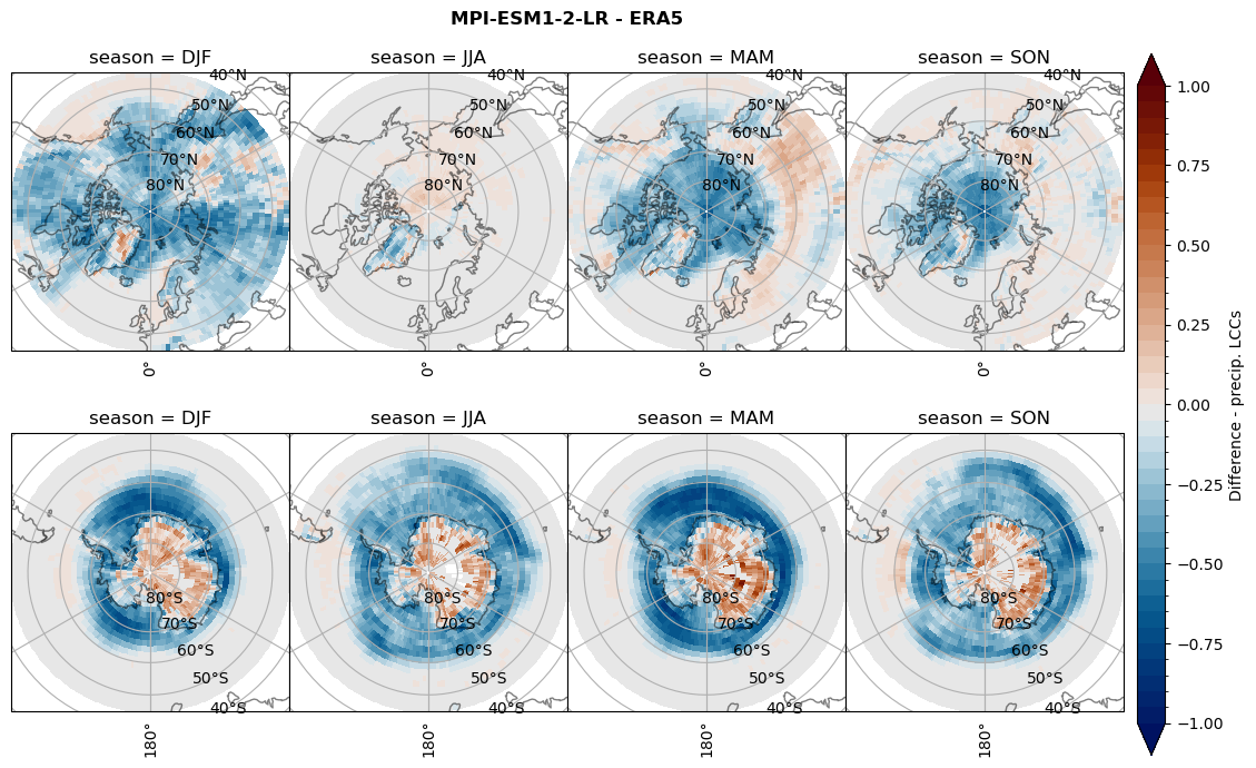
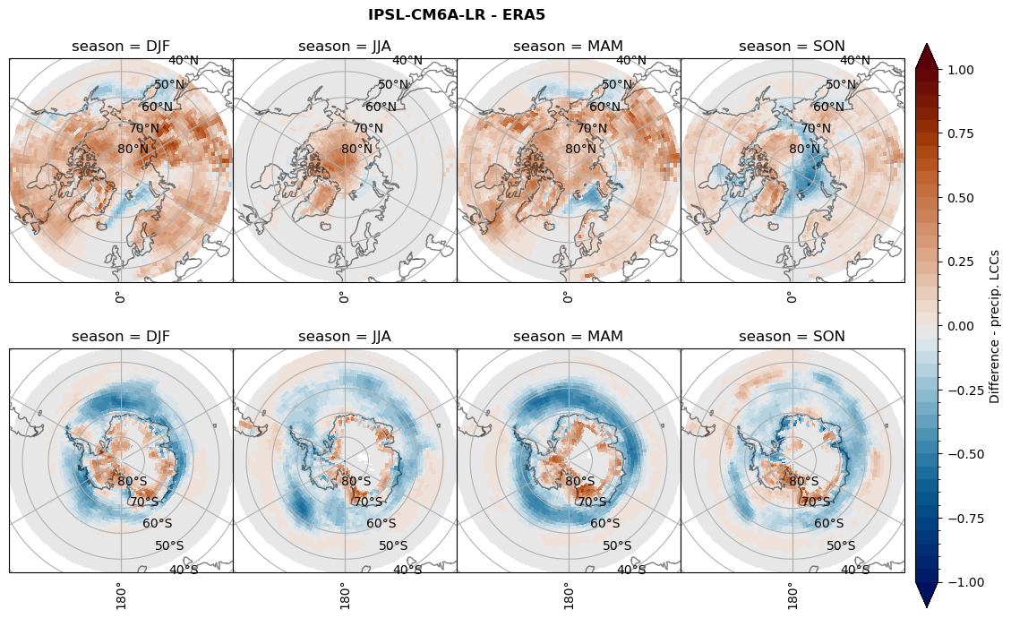
    # Difference relative frequency precipitating LCCs
    rf_lcc = dset_dict[model]['rf_lcc'] - ds_era[model]['rf_lcc']
    plt_title = '{} - ERA5'.format(model)
    levels = np.arange(-1.0, 1.05, 0.05)
    cbar_label = 'Difference - precip. LCCs'
    
    plt_seasonal_diff(rf_lcc, levels, cbar_label, plt_title)
    
    figname = '{}_diff_rf_lcc_w_snow_season_{}_{}.png'.format(model,starty, endy)
    plt.savefig(FIG_DIR + figname, format = 'png', bbox_inches = 'tight', transparent = False)

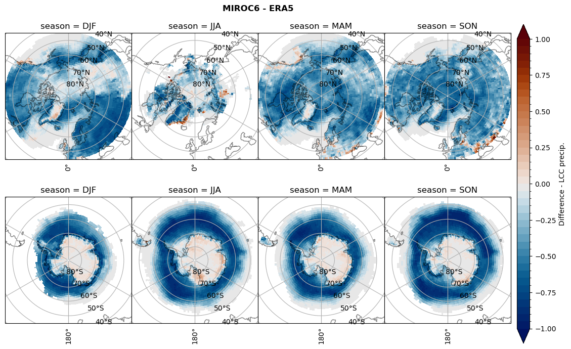
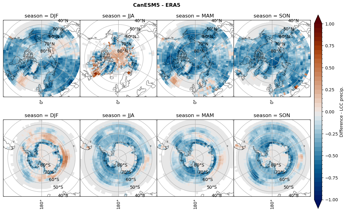
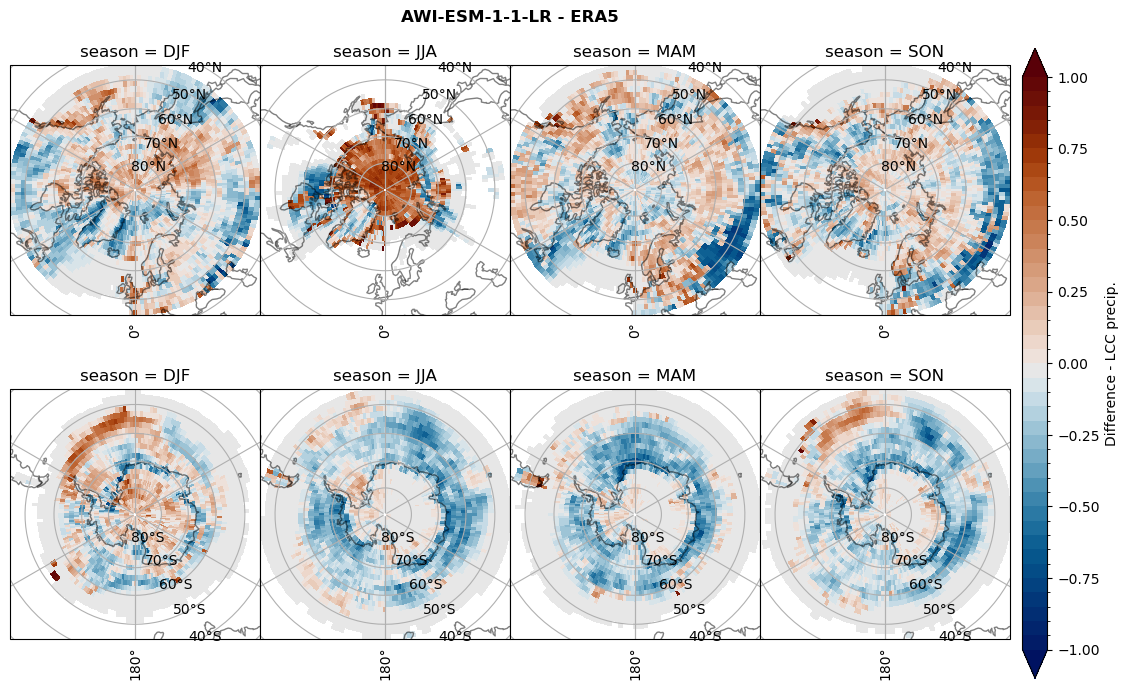
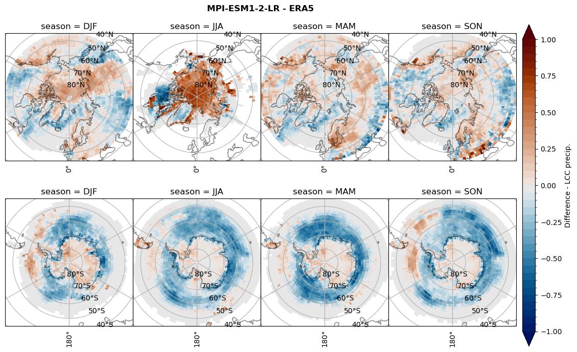
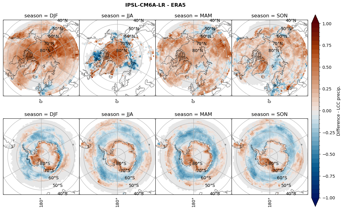
    # Difference relative frequency precipitation from LCCss
    rf_sf_lcc = dset_dict[model]['rf_sf_lcc'] - ds_era[model]['rf_sf_lcc']
    plt_title = '{} - ERA5'.format(model)
    levels = np.arange(-1.0, 1.05, 0.05)
    cbar_label = 'Difference - LCC precip.'
    
    plt_seasonal_diff(rf_sf_lcc, levels, cbar_label, plt_title)
    
    figname = '{}_diff_rf_sf_lcc_season_{}_{}.png'.format(model,starty, endy)
    plt.savefig(FIG_DIR + figname, format = 'png', bbox_inches = 'tight', transparent = False)

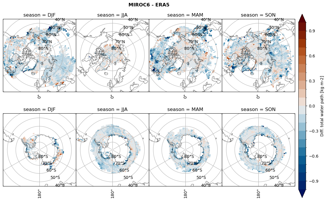
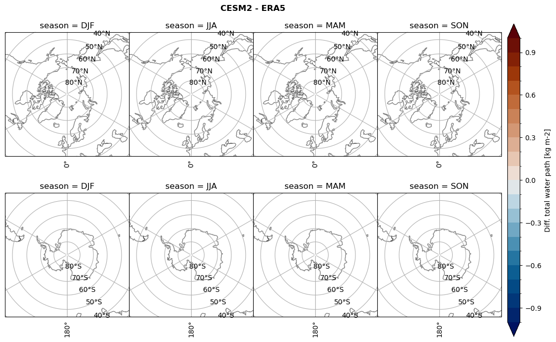
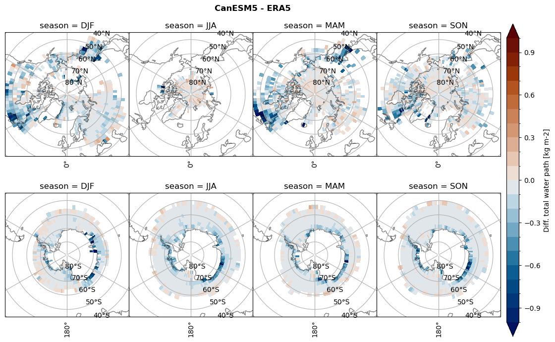
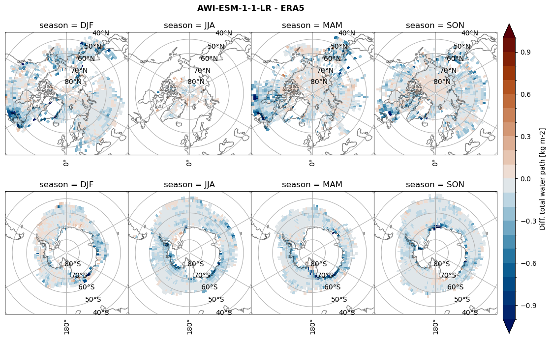
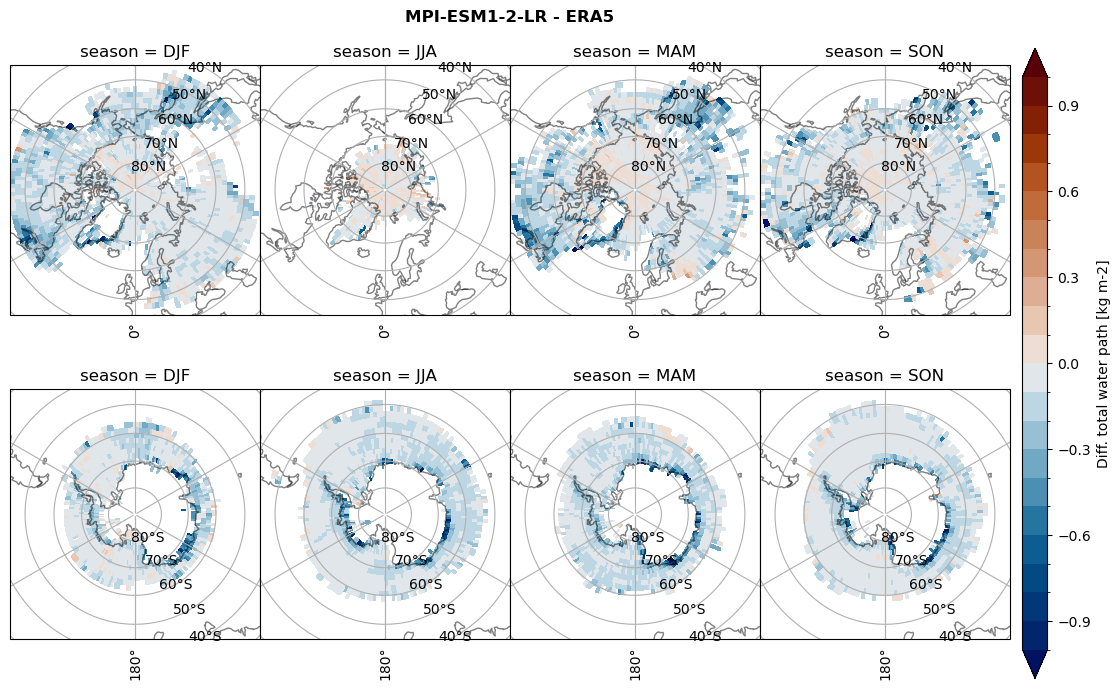
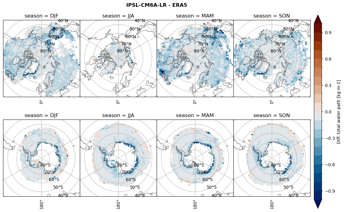
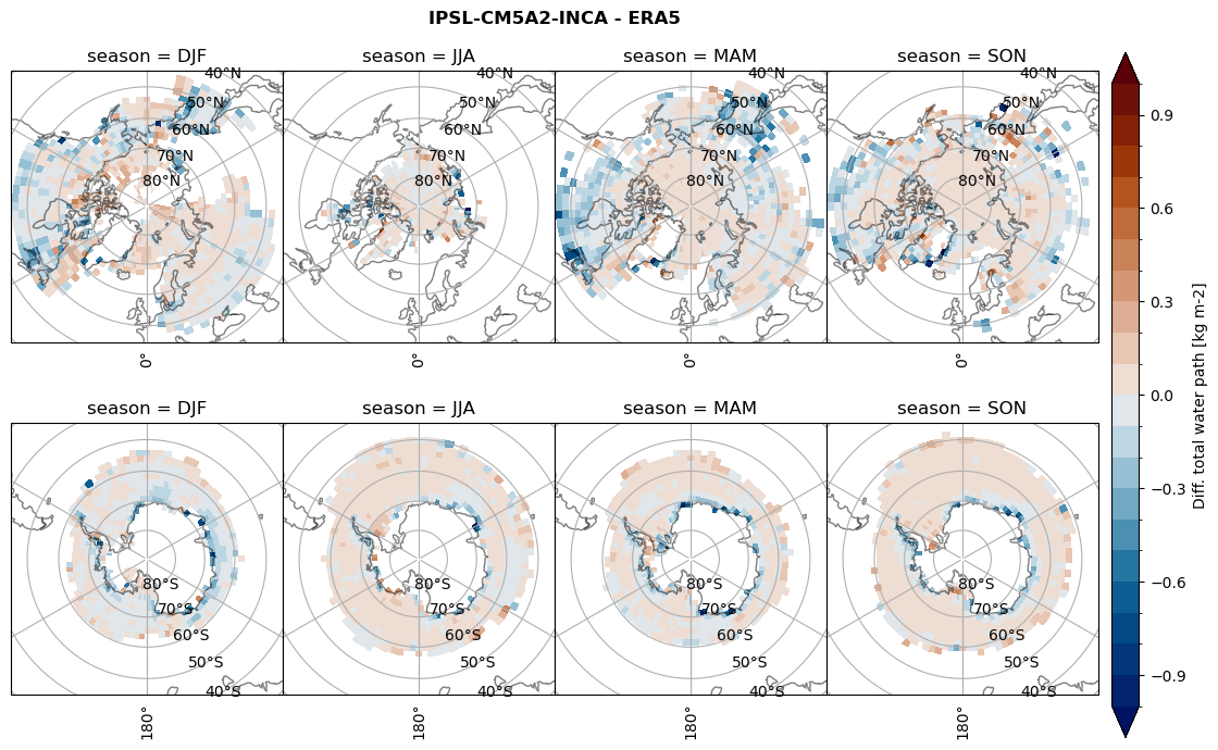
Difference total water path

for model in dset_dict.keys():

    levels = np.arange(-1,1.1,0.1)
    
    # total water path
    ds_era[model]['twp_lcc'] = ds_era[model]['iwp_lcc'] + ds_era[model]['lwp_lcc']
    variable = (dset_dict[model]['twp_lcc'] - ds_era[model]['twp_lcc']).groupby('time.season').mean('time', skipna=True, keep_attrs=True)
    
    plt_seasonal_diff(variable, levels, 'Diff. total water path [kg m-2]', '{} - ERA5'.format(model))
    figname = '{}_diff_twp_sf_days_season_mean_{}_{}.png'.format(model,starty, endy)
    plt.savefig(FIG_DIR + figname, format = 'png', bbox_inches = 'tight', transparent = False)
    
    
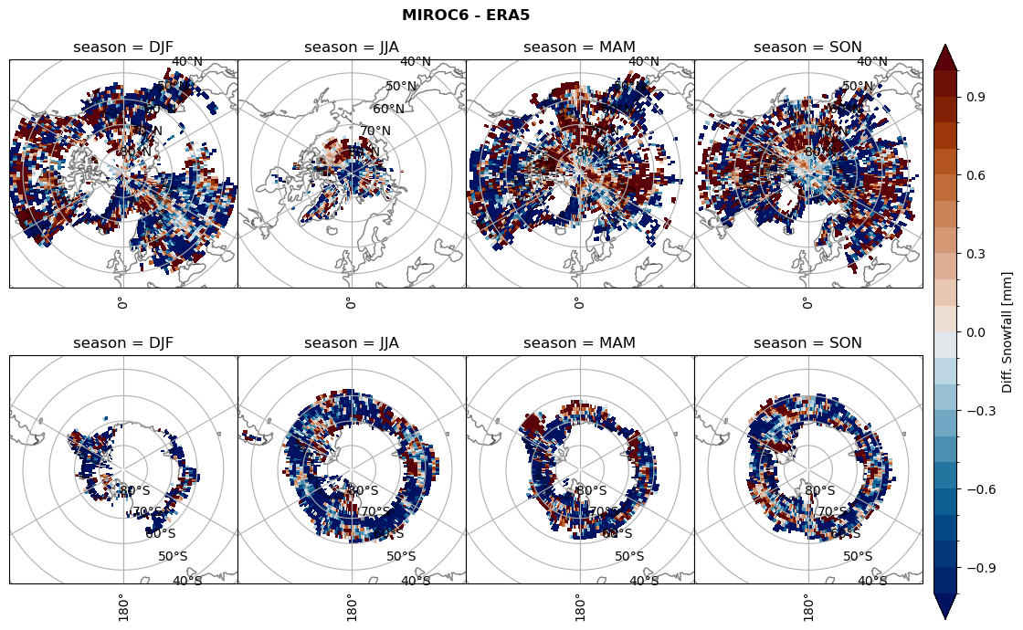
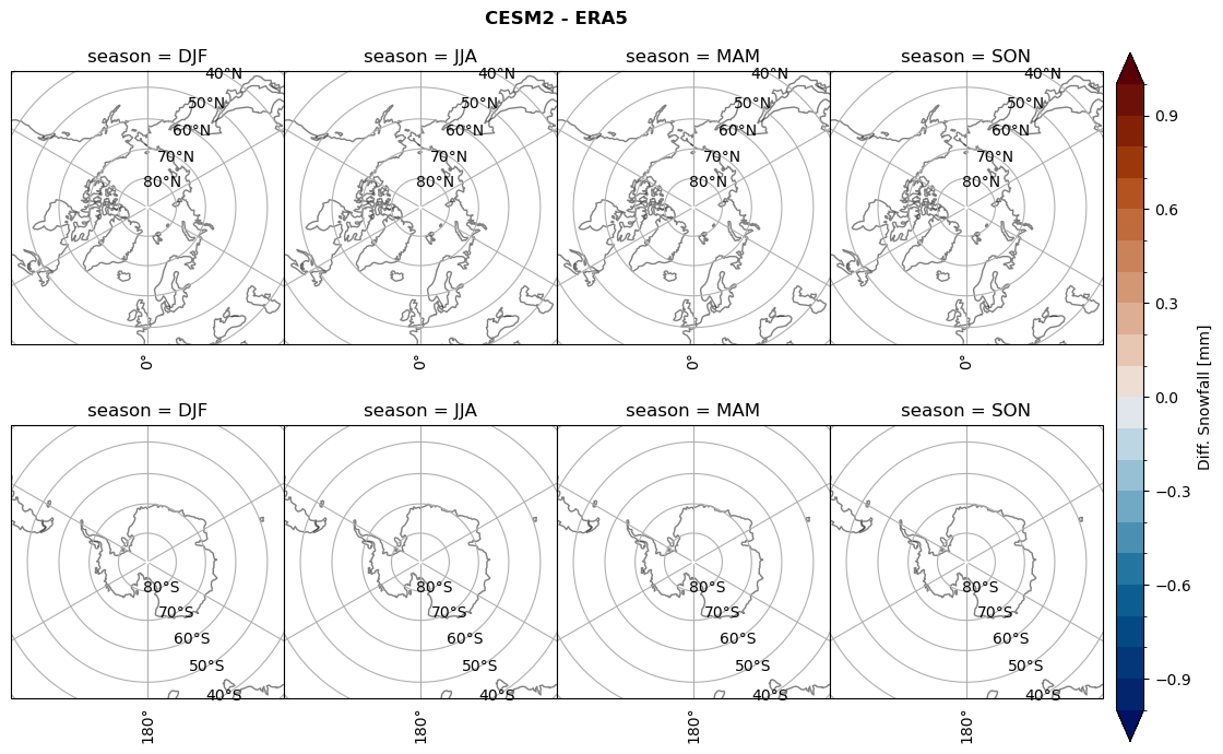
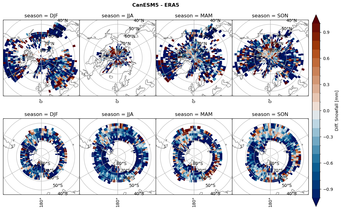
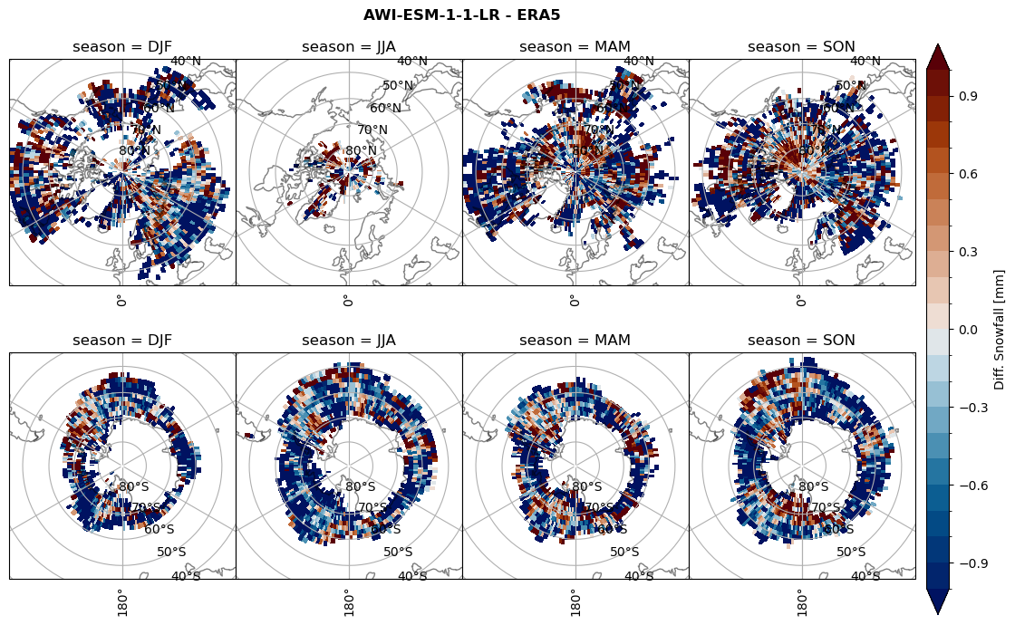
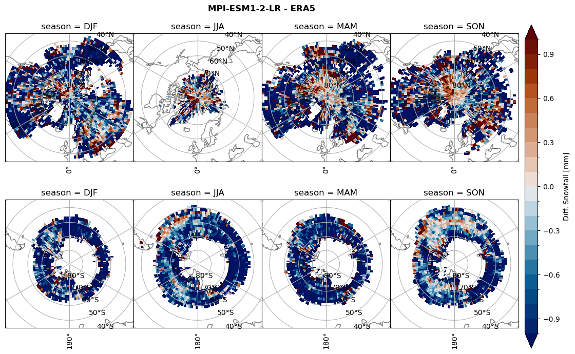
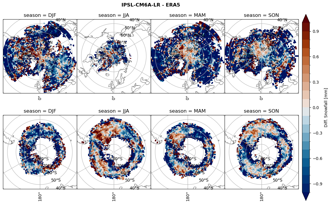
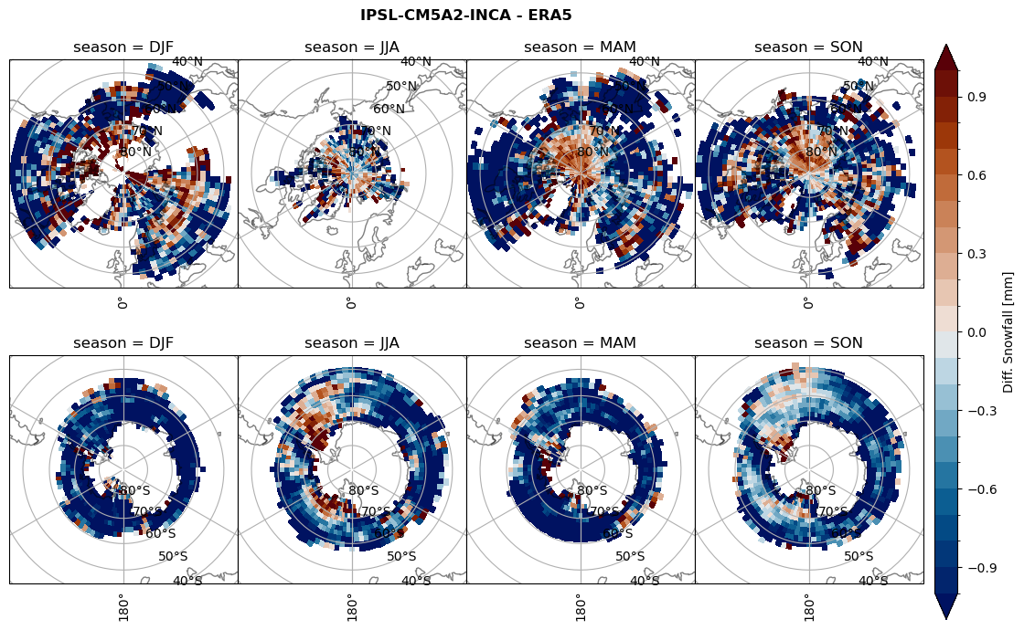
    # snowfall difference for snowfall days
    variable = (dset_dict[model]['sf_lcc'] - ds_era[model]['sf_lcc']).groupby('time.season').mean('time', skipna=True, keep_attrs=True)    
    plt_seasonal_diff(variable, levels, 'Diff. Snowfall [mm]', '{} - ERA5'.format(model))
    figname = '{}_diff_sf_sf_days_season_mean_{}_{}.png'.format(model,starty, endy)
    plt.savefig(FIG_DIR + figname, format = 'png', bbox_inches = 'tight', transparent = False)

Calendar

Not all models in CMIP6 use the same calendar. Hence we double check the time axis. Later, when we regrid to the same horizontal resolution (Regrid CMIP6 data) we will assign the same calendars for each model.

# # metadata of the historical run:
# _d2 = pd.Series(["calendar",
#                  "branch_time_in_parent", #"parent_activity_id", "parent_experiment_id",	"parent_mip_era",
#                  "parent_source_id",#"parent_sub_experiment_id", 
#                  "parent_time_units",# "parent_variant_label"
#                   ])
# _d2 = pd.DataFrame(_d2).rename(columns={0:'index'})
# for model in dset_dict.keys():
#     _data = []
#     _names =[]
#     _data.append(dset_dict[model].time.to_index().calendar)
#     for k, v in dset_dict[model].attrs.items():
        
#         if 'parent_time_units' in k or 'branch_time_in_parent' in k or 'parent_source_id' in k:
#             _data.append(v)
#             _names.append(k)
#     _d2 = pd.concat([_d2,   pd.Series(_data)], axis=1)

# _d2.dropna(how='all', axis=1, inplace=True)
# _d2 = _d2.set_index('index')
# _d2.columns = _d2.loc['parent_source_id']
# _d2.drop('parent_source_id').T

Show attributes and individual identifier

… is going to be the reference model for the horizontal grid. The xarray datasets inside dset_dict can be extracted as any value in a Python dictionary.

The dictonary key is the source_id from list_models.

# for model in dset_dict.keys():
#     print('Institution: {}, \
#           Model: {},   \
#           Nominal res: {},  \
#           lon x lat, level, top,: {}, \
#           tracking_id: {}'.format(dset_dict[model].attrs['institution_id'],
#                                   dset_dict[model].attrs['source_id'], 
#                                   dset_dict[model].attrs['nominal_resolution'], 
#                                   dset_dict[model].attrs['source'],
#                                   dset_dict[model].attrs['tracking_id']))

Assign attributes to the variables

We will assign the attributes to the variables as in ERA5 to make CMIP6 and ERA5 variables comperable.

• pr and prsn in kg m-2 s-1 \(\rightarrow\) Multiply by 3600 to get mm h-1

# now = datetime.utcnow()
# for model in dset_dict.keys():
# # 
#     for var_id in dset_dict[model].keys():
         
#         if var_id == 'prsn':
#             dset_dict[model][var_id] = dset_dict[model][var_id]*3600
#             dset_dict[model][var_id] = dset_dict[model][var_id].assign_attrs({'standard_name': 'snowfall_flux',
#     'long_name': 'Snowfall Flux',
#     'comment': 'At surface; includes precipitation of all forms of water in the solid phase',
#     'units': 'mm h-1',
#     'original_units': 'kg m-2 s-1',
#     'history': "{}Z altered by F. Hellmuth: Converted units from 'kg m-2 s-1' to 'mm h-1'.".format(now.strftime("%d/%m/%Y %H:%M:%S")),
#     'cell_methods': 'area: time: mean',
#     'cell_measures': 'area: areacella'})

Interpolate from CMIP6 hybrid sigma-pressure levels to ERA5 isobaric pressure levels

The vertical variables in the CMIP6 models are in hybrid sigma-pressure levels. Hence the vertical variable in the xarray datasets in dset_dict will be calculated by using the formula: $\( P(i,j,k) = hyam(k) p0 + hybm(k) ps(i,j)\)$ to calculate the pressure

# # Rename datasets with different naming convention for constant hyam
# for model in dset_dict.keys():
#     if ('a' in list(dset_dict[model].keys())) == True:
#         dset_dict[model] = dset_dict[model].rename({'a':'ap', 'a_bnds': 'ap_bnds'})
#     if model == 'IPSL-CM6A-LR':
#         dset_dict[model] = dset_dict[model].rename({'presnivs':'plev'})
#     if model == 'IPSL-CM5A2-INCA':
#         dset_dict[model] = dset_dict[model].rename({'lev':'plev'})
    

# for model in dset_dict.keys():
#     for var_id in dset_dict[model].keys():#['clw', 'cli']:
#         if var_id == 'clw' or var_id == 'cli':
#             # Convert the model level to isobaric levels
#             #### ap, b, ps, p0
#             if ('ap' in list(dset_dict[model].keys())) == True and \
#                 ('ps' in list(dset_dict[model].keys())) == True and \
#                 ('p0' in list(dset_dict[model].keys())) == True:
#                 if ('lev' in list(dset_dict[model][var_id].coords)) == True and \
#                     ('lev' in list(dset_dict[model]['ap'].coords)) == True and \
#                     ('lev' in list(dset_dict[model]['b'].coords)) == True:
#                         print(model, var_id, 'lev, ap, ps, p0')
#                         # dset_dict[model][var_id] = gc.interpolation.interp_hybrid_to_pressure(data = dset_dict[model][var_id],
#                         #                                                                                 ps   = dset_dict[model]['ps'], 
#                         #                                                                                 hyam = dset_dict[model]['ap'], 
#                         #                                                                                 hybm = dset_dict[model]['b'], 
#                         #                                                                                 p0   = dset_dict[model]['p0'], 
#                         #                                                                                 new_levels=new_levels,
#                         #                                                                                 lev_dim='lev')
#                         dset_dict[model]['plev'] = dset_dict[model]['ap']*dset_dict[model]['p0'] + dset_dict[model]['b']*dset_dict[model]['ps']
#                         dset_dict[model]['plev'] = dset_dict[model]['plev'].transpose('time', 'lev','lat','lon')
                
#                 if ('plev' in list(dset_dict[model][var_id].coords)) == True:
#                     print(model, var_id, 'variable on pressure levels', )
#                 # if ('lev' in list(dset_dict[model][var_id].coords)) == True and \
#                 #     ('lev' in list(dset_dict[model]['ap'].coords)) == False and \
#                 #     ('lev' in list(dset_dict[model]['b'].coords)) == False:
#                 #         print(model, 'variable on pressure levels', 'lev, ap, ps,')
#             # Convert the model level to isobaric levels
#             #### ap, b, p0
#             if ('ap' in list(dset_dict[model].keys())) == True and \
#                 ('ps' in list(dset_dict[model].keys())) == True and \
#                 ('p0' in list(dset_dict[model].keys())) == False:
#                 if ('lev' in list(dset_dict[model][var_id].coords)) == True and \
#                     ('lev' in list(dset_dict[model]['ap'].coords)) == True and \
#                     ('lev' in list(dset_dict[model]['b'].coords)) == True:
#                         print(model,var_id, 'lev, ap, ps,')
#                         # dset_dict[model][var_id] = gc.interpolation.interp_hybrid_to_pressure(data = dset_dict[model][var_id],
#                         #                                                                                 ps   = dset_dict[model]['ps'], 
#                         #                                                                                 hyam = dset_dict[model]['ap'], 
#                         #                                                                                 hybm = dset_dict[model]['b'], 
#                         #                                                                                 new_levels=new_levels,
#                         #                                                                                 lev_dim='lev')
#                         dset_dict[model]['plev'] = dset_dict[model]['ap'] + dset_dict[model]['b']*dset_dict[model]['ps']
#                         dset_dict[model]['plev'] = dset_dict[model]['plev'].transpose('time', 'lev','lat','lon')
                
#                 if ('plev' in list(dset_dict[model][var_id].coords)) == True:
#                     print(model, var_id, 'variable on pressure levels', )
                
#             if ('b' in list(dset_dict[model].keys())) == True and \
#                 ('orog' in list(dset_dict[model].keys())) == True:
#                 if ('lev' in list(dset_dict[model][var_id].coords)) == True and \
#                     ('lev' in list(dset_dict[model]['pfull'].coords)) == True:
#                         print(model, 'hybrid height coordinate')
                

Calculate liquid water path from content

# for model in dset_dict.keys():
    
#     if ('plev' in list(dset_dict[model].keys())) == True:
#         print(model, 'plev')
#         _lwp = xr.DataArray(data=da.full(shape=dset_dict[model]['clw'].shape,fill_value=np.nan),
#                                 dims=dset_dict[model]['clw'].dims,
#                                 coords=dset_dict[model]['clw'].coords)
#         # lev2 is the atmospheric pressure, lower in the atmosphere than lev. Sigma-pressure coordinates are from 1 to 0, with 1 at the surface
#         for i in range(len(dset_dict[model]['lev'])-1):
#             # calculate pressure difference between two levels
#             dp = (dset_dict[model]['plev'].isel(lev=i) - dset_dict[model]['plev'].isel(lev=i+1))
#             # calculate mean liquid water content between two layers
#             dlwc = (dset_dict[model]['clw'].isel(lev=i) + dset_dict[model]['clw'].isel(lev=i+1))/2
#             # calculate liquid water path between two layers
#             _lwp[:,i,:,:] = dp[:,:,:]/9.81 * dlwc[:,:,:]
        
#             # sum over all layers to ge the liquid water path in the atmospheric column
#             dset_dict[model]['lwp'] = _lwp.sum(dim='lev',skipna=True)
            
#             # assign attributes to data array
#             dset_dict[model]['lwp'] = dset_dict[model]['lwp'].assign_attrs(dset_dict[model]['clw'].attrs)
#             dset_dict[model]['lwp'] = dset_dict[model]['lwp'].assign_attrs({'long_name':'Liquid Water Path', 
#                                                                             'units' : 'kg m-2',
#                                                                                 'mipTable':'', 'out_name': 'lwp',
#                                                                                 'standard_name': 'atmosphere_mass_content_of_cloud_liquid_water',
#                                                                                 'title': 'Liquid Water Path',
#                                                                                 'variable_id': 'lwp', 'original_units': 'kg/kg',
#                                                                                 'history': "{}Z altered by F. Hellmuth: Interpolate data from hybrid-sigma levels to isobaric levels with P=a*p0 + b*psfc. Calculate lwp with hydrostatic equation.".format(now.strftime("%d/%m/%Y %H:%M:%S"))})
#         # when ice water path does not exist
#         if ('clivi' in list(dset_dict[model].keys())) == False:
#             _iwp = xr.DataArray(data=da.full(shape=dset_dict[model]['cli'].shape,fill_value=np.nan),
#                                     dims=dset_dict[model]['cli'].dims,
#                                     coords=dset_dict[model]['cli'].coords)
#             # lev2 is the atmospheric pressure, lower in the atmosphere than lev. Sigma-pressure coordinates are from 1 to 0, with 1 at the surface
#             for i in range(len(dset_dict[model]['lev'])-1):
#                 # calculate pressure difference between two levels
#                 dp = (dset_dict[model]['plev'].isel(lev=i) - dset_dict[model]['plev'].isel(lev=i+1))
#                 # calculate mean liquid water content between two layers
#                 diwc = (dset_dict[model]['cli'].isel(lev=i) + dset_dict[model]['cli'].isel(lev=i+1))/2
#                 # calculate liquid water path between two layers
#                 _iwp[:,i,:,:] = dp[:,:,:]/9.81 * diwc[:,:,:]
            
                
#                 # sum over all layers to ge the Ice water path in the atmospheric column
#                 dset_dict[model]['clivi'] = _iwp.sum(dim='lev',skipna=True)
                
#                 # assign attributes to data array
#                 dset_dict[model]['clivi'] = dset_dict[model]['clivi'].assign_attrs(dset_dict[model]['cli'].attrs)
#                 dset_dict[model]['clivi'] = dset_dict[model]['clivi'].assign_attrs({'long_name':'Ice Water Path', 
#                                                                                 'units' : 'kg m-2',
#                                                                                     'mipTable':'', 'out_name': 'clivi',
#                                                                                     'standard_name': 'atmosphere_mass_content_of_cloud_ice_water',
#                                                                                     'title': 'Ice Water Path',
#                                                                                     'variable_id': 'clivi', 'original_units': 'kg/kg',
#                                                                                     'history': "{}Z altered by F. Hellmuth: Interpolate data from hybrid-sigma levels to isobaric levels with P=a*p0 + b*psfc. Calculate clivi with hydrostatic equation.".format(now.strftime("%d/%m/%Y %H:%M:%S"))})
            
#     if ('plev' in list(dset_dict[model].coords)) == True:
#         print(model, 'plev coord')
#         _lwp = xr.DataArray(data=da.full(shape=dset_dict[model]['clw'].shape,fill_value=np.nan),
#                                 dims=dset_dict[model]['clw'].dims,
#                                 coords=dset_dict[model]['clw'].coords)
#         # lev2 is the atmospheric pressure, lower in the atmosphere than lev. Sigma-pressure coordinates are from 1 to 0, with 1 at the surface
#         for i in range(len(dset_dict[model]['plev'])-1):
#             # calculate pressure difference between two levels
#             dp = (dset_dict[model]['plev'].isel(plev=i) - dset_dict[model]['plev'].isel(plev=i+1))
#             # calculate mean liquid water content between two layers
#             dlwc = (dset_dict[model]['clw'].isel(plev=i) + dset_dict[model]['clw'].isel(plev=i+1))/2
#             # calculate liquid water path between two layers
#             _lwp[:,i,:,:] = dp/9.81 * dlwc[:,:,:]
        
#             # sum over all layers to ge the liquid water path in the atmospheric column
#             dset_dict[model]['lwp'] = _lwp.sum(dim='plev',skipna=True)
            
#             # assign attributes to data array
#             dset_dict[model]['lwp'] = dset_dict[model]['lwp'].assign_attrs(dset_dict[model]['clw'].attrs)
#             dset_dict[model]['lwp'] = dset_dict[model]['lwp'].assign_attrs({'long_name':'Liquid Water Path', 
#                                                                             'units' : 'kg m-2',
#                                                                                 'mipTable':'', 'out_name': 'lwp',
#                                                                                 'standard_name': 'atmosphere_mass_content_of_cloud_liquid_water',
#                                                                                 'title': 'Liquid Water Path',
#                                                                                 'variable_id': 'lwp', 'original_units': 'kg/kg',
#                                                                                 'history': "{}Z altered by F. Hellmuth: Interpolate data from hybrid-sigma levels to isobaric levels with P=a*p0 + b*psfc. Calculate lwp with hydrostatic equation.".format(now.strftime("%d/%m/%Y %H:%M:%S"))})
#         # when ice water path does not exist
#         if ('clivi' in list(dset_dict[model].keys())) == False:
#             _iwp = xr.DataArray(data=da.full(shape=dset_dict[model]['cli'].shape,fill_value=np.nan),
#                                     dims=dset_dict[model]['cli'].dims,
#                                     coords=dset_dict[model]['cli'].coords)
#             # lev2 is the atmospheric pressure, lower in the atmosphere than lev. Sigma-pressure coordinates are from 1 to 0, with 1 at the surface
#             for i in range(len(dset_dict[model]['plev'])-1):
#                 # calculate pressure difference between two levels
#                 dp = (dset_dict[model]['plev'].isel(plev=i) - dset_dict[model]['plev'].isel(plev=i+1))
#                 # calculate mean liquid water content between two layers
#                 diwc = (dset_dict[model]['cli'].isel(plev=i) + dset_dict[model]['cli'].isel(plev=i+1))/2
#                 # calculate liquid water path between two layers
#                 _iwp[:,i,:,:] = dp/9.81 * diwc[:,:,:]
            
                
#                 # sum over all layers to ge the Ice water path in the atmospheric column
#                 dset_dict[model]['clivi'] = _iwp.sum(dim='plev',skipna=True)
                
#                 # assign attributes to data array
#                 dset_dict[model]['clivi'] = dset_dict[model]['clivi'].assign_attrs(dset_dict[model]['clw'].attrs)
#                 dset_dict[model]['clivi'] = dset_dict[model]['clivi'].assign_attrs({'long_name':'Ice Water Path', 
#                                                                                 'units' : 'kg m-2',
#                                                                                     'mipTable':'', 'out_name': 'clivi',
#                                                                                     'standard_name': 'atmosphere_mass_content_of_cloud_ice_water',
#                                                                                     'title': 'Ice Water Path',
#                                                                                     'variable_id': 'clivi', 'original_units': 'kg/kg',
#                                                                                     'history': "{}Z altered by F. Hellmuth: Interpolate data from hybrid-sigma levels to isobaric levels with P=a*p0 + b*psfc. Calculate clivi with hydrostatic equation.".format(now.strftime("%d/%m/%Y %H:%M:%S"))})
            

# lwp_count_month = dset_dict[model]['lwp_lcc'].groupby('time.month').count(dim='time')
# lwp_count_season = dset_dict[model]['lwp'].groupby('time.season').count(dim='time')

# lcc_freq_djf = (lwp_count_month.sel(month=12)+lwp_count_month.sel(month=1)+lwp_count_month.sel(month=2)) / lwp_count_season.sel(season='DJF')
# lcc_freq_mam = (lwp_count_month.sel(month=3) + lwp_count_month.sel(month=4) + lwp_count_month.sel(month=5)) / lwp_count_season.sel(season='MAM')
# lcc_freq_jja = (lwp_count_month.sel(month=6) + lwp_count_month.sel(month=7) + lwp_count_month.sel(month=8)) / lwp_count_season.sel(season='JJA')
# lcc_freq_son = (lwp_count_month.sel(month=9) + lwp_count_month.sel(month=10) + lwp_count_month.sel(month=11)) / lwp_count_season.sel(season='SON')

# lcc_freq = xr.concat([lcc_freq_djf, lcc_freq_mam, lcc_freq_jja, lcc_freq_son], dim='season')

# plt_seasonal_NH_SH(lcc_freq, np.arange(0,1.1,0.1), 'LCC frequency', model)

Open CMIP6 variables

… by using intake from pangeo.io, specifically intake-esm.

An example on Loading an ESM collection and searching for datasets can also be found on the Pangeo / ESGF Cloud Data Working Group documentation.

# cat_url = "https://storage.googleapis.com/cmip6/pangeo-cmip6.json"
# col = intake.open_esm_datastore(cat_url)
# col

Search corresponding data

Get the data required for the analysis. Define variables, models, experiment, and time resolution as defined in 2. Data Wrangling .

• use member_id = ‘r1i1p1f1’.

• using intake-esm’s search() function:

  • col.search(variable_id, source_id, experiment_id, table_id, member_id, institution_id, grid_label)

# ## Variables
# variable_id=[
#             'cli',
#             'clivi',
#             'clw',
#             # 'lwp',
#             # 'pr',
#             'prsn',
#             # 'ta', 
#             'tas'
#              ]

# ## Models
# # list_models = [
# #     'NorESM2-MM',
# #     'TaiESM1',
# #     'EC-Earth3-AerChem',
# #     'GFDL-ESM4',
# #     'SAM0-UNICON',
# #     'CAMS-CSM1-0',
# #     'CMCC-CM2-HR4',
# #     'MPI-ESM1-2-HR',
# #     'BCC-CSM2-MR',
# #     'E3SM-1-1',
# #     'CMCC-CM2-SR5',
# #     'CMCC-ESM2',
# #     'FGOALS-f3-L',
# #     'E3SM-1-1-ECA',
# #     'CIESM',
# #     'GFDL-CM4',
# #     'MRI-ESM2-0']  

# list_models = ['MIROC6', 'CESM2', 'CanESM5', 'AWI-ESM-1-1-LR', 'MPI-ESM1-2-LR',
#        'UKESM1-0-LL', 'HadGEM3-GC31-LL', 'CNRM-CM6-1', 'CNRM-ESM2-1',
#        'IPSL-CM6A-LR', 'IPSL-CM5A2-INCA']

# ## experiment
# experiment_id = ['historical']

# ## time resolution
# t_res = ['day', 'CFday']

# ## search for variables, models, ...
# cat = col.search(variable_id=variable_id, source_id=list_models, experiment_id=experiment_id, table_id = t_res, member_id=['r1i1p1f1'])
# # cat.df
# ## show the CMIP6 models found in pandas Dataframe 
# cat.df['source_id'].unique()

Create dictionary from the list of datasets we found

Load the found datasets into xarray dataset containers using intake-esm’s to_dataset_dict() function, which yields a Python dictionary.

NOTE: This step may take several minutes so be patient!

# dset_dict = cat.to_dataset_dict(zarr_kwargs={'use_cftime':True,})

# dset_dict.keys()

# # list all merged datasets and show coordinates
# for keys, ds in dset_dict.items():
#     print('{}: {}'.format(keys, list(ds.dims)))

Calendar

Not all models in CMIP6 use the same calendar. Hence we double check the time axis. Later, when we regrid to the same horizontal resolution (Regrid CMIP6 data) we will assign the same calendars for each model.

# # metadata of the historical run:
# _d2 = pd.Series(["calendar",
#                  "branch_time_in_parent", #"parent_activity_id", "parent_experiment_id",	"parent_mip_era",
#                  "parent_source_id",#"parent_sub_experiment_id", 
#                  "parent_time_units",# "parent_variant_label"
#                   ])
# _d2 = pd.DataFrame(_d2).rename(columns={0:'index'})
# for i in dset_dict.keys():
#     _data = []
#     _names =[]
#     _data.append(dset_dict[i].time.to_index().calendar)
#     for k, v in dset_dict[i].attrs.items():
        
#         if 'parent_time_units' in k or 'branch_time_in_parent' in k or 'parent_source_id' in k:
#             _data.append(v)
#             _names.append(k)
#     _d2 = pd.concat([_d2,   pd.Series(_data)], axis=1)

# _d2.dropna(how='all', axis=1, inplace=True)
# _d2 = _d2.set_index('index')
# _d2.columns = _d2.loc['parent_source_id']
# _d2.drop('parent_source_id').T

Show attributes and individual identifier

NorESM2-MM is going to be the reference model for the horizontal grid. The xarray datasets inside dset_dict can be extracted as any value in a Python dictionary.

The dictonary key for NorESM2-MM is: CMIP.NCC.NorESM2-MM.historical.Amon.gn

# if variable_id[0] == 'lwp':
#     ds = dset_dict['CMIP.NCC.NorESM2-MM.historical.AERmon.gn']
# else:
#     ds = dset_dict['CMIP.NCC.NorESM2-MM.historical.Amon.gn']
    

## attributes of the xarray dataset 
# ds[variable_id[0]].attrs, ds.attrs['tracking_id']

# dset_dict.keys()

# for model in dset_dict.keys():
#     for keys in dset_dict[model].keys():
#         print(model, keys)

Assign attributes to the variables

We will assign the attributes to the variables as in ERA5 to make CMIP6 and ERA5 variables comperable.

• cli and clw in kg kg-1 \(\rightarrow\) Multiply by 1000 to get g kg-1

• clivi and lwp in kg m-2 \(\rightarrow\) Multiply by 1000 to get g m-2

• pr and prsn in kg m-2 s-1 \(\rightarrow\) Multiply by 86400 to get mm day-1

# for var_id in variable_id:
#     for keys in dset_dict.keys():
#         if var_id == 'cli' or var_id == 'clw' or var_id == 'lwp' or var_id  == 'clivi':
#             dset_dict[keys][var_id] = dset_dict[keys][var_id]*1000
#             if var_id == 'cli':
#                 dset_dict[keys][var_id].attrs = {'units': 'g kg-1', 'long_name': 'Mass Fraction of Cloud Ice', 'standard_name': 'mass_fraction_of_cloud_ice_in_air', 'comment': 'Includes both large-scale and convective cloud. This is calculated as the mass of cloud ice in the grid cell divided by the mass of air (including the water in all phases) in the grid cell. It includes precipitating hydrometeors ONLY if the precipitating hydrometeors affect the calculation of radiative transfer in model.', 'cell_methods': 'area: time: mean (interval: 5 minutes)', 'cell_measures': 'area: areacella',}
#             if var_id == 'clw':
#                 dset_dict[keys][var_id].attrs = {'units': 'g kg-1', 'long_name': 'Mass Fraction of Cloud Liquid Water', 'standard_name': 'mass_fraction_of_cloud_liquid_water_in_air', 'comment': 'Includes both large-scale and convective cloud. Calculate as the mass of cloud liquid water in the grid cell divided by the mass of air (including the water in all phases) in the grid cells. Precipitating hydrometeors are included ONLY if the precipitating hydrometeors affect the calculation of radiative transfer in model.', 'cell_methods': 'area: time: mean', 'cell_measures': 'area: areacella'}
#             if var_id == 'clivi':
#                 dset_dict[keys][var_id].attrs = {'units': 'g m-2', 'long_name': 'Ice Water Path', 'comment': 'mass of ice water in the column divided by the area of the column (not just the area of the cloudy portion of the column). Includes precipitating frozen hydrometeors ONLY if the precipitating hydrometeor affects the calculation of radiative transfer in model.', 'cell_methods': 'area: time: mean', 'cell_measures': 'area: areacella'} 
#             if var_id == 'lwp':
#                 dset_dict[keys][var_id].attrs = {'units': 'g m-2', 'long_name': 'Liquid Water Path', 'comment': 'The total mass of liquid water in cloud per unit area.', 'cell_methods': 'area: time: mean', 'cell_measures': 'area: areacella'}

#         if var_id == 'pr' or var_id == 'prsn':
#             try: 
#                 dset_dict[keys][var_id] = dset_dict[keys][var_id]*86400
#                 if var_id == 'pr':
#                     dset_dict[keys][var_id].attrs = {'units': 'mm day-1', 'long_name': 'Precipitation', 'comment': 'includes both liquid and solid phases','cell_methods': 'area: time: mean', 'cell_measures': 'area: areacella'}
#                 if var_id == 'prsn':
#                     dset_dict[keys][var_id].attrs = {'units': 'mm day-1', 'long_name': 'Snowfall', 'comment': 'At surface; includes precipitation of all forms of water in the solid phase', 'cell_methods': 'area: time: mean', 'cell_measures': 'area: areacella'}
#             except KeyError:
#                 continue
        

Interpolate from CMIP6 hybrid sigma-pressure levels to ERA5 isobaric pressure levels

The vertical variables in the CMIP6 models are in hybrid sigma-pressure levels. Hence the vertical variable in the xarray datasets in dset_dict will be calculated by using the GeoCAT-comb function to interpolate data from hybrid-sigma levels to isobaric levels.

The GeoCAT-comb function takes the following input:

• data: Multidimensional data array, which holds hybrid-sigma levels and has a lev_dim coordinate.

• ps: A multi-dimensional array of surface pressures (Pa), same time/space shape as data. Not all variables include the surface pressure, hence we will search the Pangeo.io catalog to find the surface pressure associated with the model.

• hyam: One-dimensional arrays containing the hybrid A coefficients. Must have the same dimension size as the lev_dim dimension of data.

• hybm: One-dimensional arrays containing the hybrid B coefficients. Must have the same dimension size as the lev_dim dimension of data.

• p0: Scalar numeric value equal to surface reference pressure (Pa). Defaults to 100000 Pa.

• new_levels: A one-dimensional array of output pressure levels (Pa). We will use the pressure of air_temperature (19 levels).

\[ P(i,j,k) = hyam(k) p0 + hybm(k) ps(i,j)\]

import geocat

geocat.comp.interpolation.interp_hybrid_to_pressure(data      =ds['variable'], 
                                                    ps        =ds['ps'], 
                                                    hyam      =ds['a'], 
                                                    hybm      =ds['b'], 
                                                    p0        =ds['p0'], 
                                                    new_levels=ds['plev'])

# # load the levels from the ERA5 file and transfer to Pa
# era_level = (xr.open_dataset('/scratch/franzihe/input/ERA5/monthly_means/0.25deg/clwc_Amon_ERA5_198501_198912.nc')['level'])*100

# if (('clw' or 'cli' or 'ta') in variable_id) == True:
#     # if var_id == 'clw' or var_id == 'cli':
#     for keys in dset_dict.keys():
#         # rename cmip pressure level for atmospheric temperature
#         dset_dict[keys] = dset_dict[keys].rename({'plev':'clev'})
#         # interpolate from hybrid to pressure levels for clw and cli
#         for var_id in [variable_id[variable_id.index('clw')], variable_id[variable_id.index('cli')]]:

#             if ('ps' in list(dset_dict[keys].keys())) == False:     # valid for models which don't provide ps in the clw or cli dataset
#                 model = keys.split('.')[2]
#                 ds_ps = col.search(source_id=model, table_id = ['Amon', ], experiment_id=['historical'], variable_id=['ps','p0', ], member_id=['r1i1p1f1']).to_dataset_dict(zarr_kwargs={'use_cftime':True,}, )
#                 dset_dict[keys].update(ds_ps[keys], )
#                 dset_dict[keys]['ps'] = dset_dict[keys]['ps'].isel(member_id = 0)
                
                
#             # Rename datasets with different naming convention for constant A
#             if ('a' in list(dset_dict[keys].keys())) == False:
#                 dset_dict[keys] = dset_dict[keys].rename({'ap':'a', 'ap_bnds': 'a_bnds'})
                    
                    
#             # Convert the model level to isobaric levels
#             #### a, b, ps, p0
#             if ('a' in list(dset_dict[keys].keys())) == True and ('b' in list(dset_dict[keys].keys())) == True and ('p0' in list(dset_dict[keys].keys())) == True and ('ps' in list(dset_dict[keys].keys())) == True:
#                 dset_dict[keys]['{}_interp'.format(var_id)] = gc.interpolation.interp_hybrid_to_pressure(data=dset_dict[keys][var_id].isel(member_id = 0), 
#                                                                                                                 ps=dset_dict[keys]['ps'],hyam=dset_dict[keys]['a'],
#                                                                                                                 hybm=dset_dict[keys]['b'],
#                                                                                                                 p0=dset_dict[keys]['p0'].values, 
#                                                                                                                 new_levels=(era_level).values, )
#                 # # remove the variables needed for the calculation of the isobaric levels. If this step is not performed, 
#                 # # the horizontal regridding will not be possible.
#                 # dset_dict[keys] = dset_dict[keys].drop(('a', 'p0', 'b', 'ps', 'a_bnds', 'b_bnds', var_id))
#                 dset_dict[keys] = dset_dict[keys].drop((var_id))
#                 dset_dict[keys] = dset_dict[keys].rename({'{}_interp'.format(var_id):var_id})

#             #### a, b, ps
#             elif ('a' in list(dset_dict[keys].keys())) == True and ('b' in list(dset_dict[keys].keys())) == True and ('ps' in list(dset_dict[keys].keys())) == True and ('p0' in list(dset_dict[keys].keys())) == False:
#                 dset_dict[keys]['{}_interp'.format(var_id)] = gc.interpolation.interp_hybrid_to_pressure(data=dset_dict[keys][var_id].isel(member_id=0), 
#                                                                                                                 ps=dset_dict[keys]['ps'],
#                                                                                                                 hyam=dset_dict[keys]['a'], 
#                                                                                                                 hybm=dset_dict[keys]['b'],
#                                                                                                                 p0=100000.0,
#                                                                                                                 new_levels=(era_level).values, )
#                 # dset_dict[keys] = dset_dict[keys].drop(('a', 'b', 'ps', 'a_bnds', 'b_bnds', var_id))
#                 dset_dict[keys] = dset_dict[keys].drop((var_id))
#                 dset_dict[keys] = dset_dict[keys].rename({'{}_interp'.format(var_id):var_id})
        
#         # remove the variables needed for the calculation of the isobaric levels. If this step is not performed, 
#         # the horizontal regridding will not be possible.
#         if ('p0' in list(dset_dict[keys].keys())) == True:
#             dset_dict[keys] = dset_dict[keys].drop(('a', 'p0', 'b', 'ps', 'a_bnds', 'b_bnds',))
#         elif ('p0' in list(dset_dict[keys].keys())) == False:
#             dset_dict[keys] = dset_dict[keys].drop(('a', 'b', 'ps', 'a_bnds', 'b_bnds',))
 

Regrid CMIP6 data to NorESM2-MM grid

We want to conduct statistical analysis at the annual and seasonal timescales to determine the biases in cloud phase and precipitation (liquid and solid) in the CMIP6 models. At the moment we have all historical data from the CMIP6 models. For this, we will have to extract the 30-year period between 1985 and 2014.

\(\rightarrow\) Define a start and end year.

The CMIP6 high resolution models have approximately a nominal resolution of 100km. But not all have identical grid spacing. Hence we will make use of the python package xesmf and the documentation on decreasing resolution, Limitations and warnings.

NorESM2-MM will be the reference grid since we want to compare the models to the ERA5 data. The ERA5 data has a nominal resolution of 0.25deg and has been regridded to the same horizontal resolution as the NorESM2-MM in the ERA5 Jupyter Notebook.

\(\rightarrow\) Define NorESM2-MM as the reference grid ds_out.

Create a new Python dictionary (ds_gridded_dict) with the regridded CMIP6 xarray datasets between 1985 an 2014. Save each regridded model to a netcdf, locally.

NOTE: This step may take several minutes!

# starty = 1985; endy = 2014
# year_range = range(starty, endy+1)

# ds_out = dset_dict['CMIP.NCC.NorESM2-MM.historical.Amon.gn']
# ds_in  = dset_dict[model]

# import xesmf

# # Regridder data
# regridder = xesmf.Regridder(ds_in, ds_out, "conservative")

# # Apply regridder to data
#  # the entire dataset can be processed at once
# ds_in_regrid = regridder(ds_in)

# # create dictionary for reggridded data
# ds_gridded_dict = dict()

# # Read in the output grid from NorESM
# if variable_id[0] == 'lwp':
#     ds_out = dset_dict['CMIP.NCC.NorESM2-MM.historical.AERmon.gn'].isel(member_id = 0)
# else:
#     ds_out = dset_dict['CMIP.NCC.NorESM2-MM.historical.Amon.gn'].isel(member_id = 0)
# ds_out = ds_out.sel(time = ds_out.time.dt.year.isin(year_range)).squeeze()


# counter = 0

# for keys in dset_dict.keys():
#     # select only models which have atmospheric monthly values
#     amon = keys.split('.')[-2]
#     if amon == 'Amon' or amon == 'AERmon': 
#         # select model name 
#         model = keys.split('.')[2]
        
#         # select where data should be saved
#         if len(variable_id) > 1:
#             filename = '{}_Amon_1deg_{}01_{}12.nc'.format(variable_id, starty, endy)
#         elif len([variable_id]) == 1:
#             filename = '{}_Amon_1deg_{}01_{}12.nc'.format(variable_id[0], starty, endy)
#         # filename = '{}_Amon_1deg_{}01_{}12.nc'.format(variable_id[0], starty, endy)
#         savepath = '/scratch/franzihe/output/CMIP6_hist/1deg/{}/'.format(model)
#         nc_out = savepath + filename
#         files = glob(nc_out)
        
#         # Input data from CMIP6 model to be regridded
#         ds_in = dset_dict[keys].isel(member_id = 0)
#         ds_in = ds_in.sel(time = ds_in.time.dt.year.isin(year_range)).squeeze()
            
#         # common time grid
#         ds_in['time'] = ds_out['time']
            

#         # Regrid data
#         ds_in_regrid = fct.regrid_data(ds_in, ds_out)


#         # Shift the longitude from 0-->360 to -180-->180 and sort by longitude and time
#         ds_in_regrid = ds_in_regrid.assign_coords(lon=(((ds_in_regrid.lon + 180) % 360) - 180)).sortby('lon').sortby('time')
#         ds_in_regrid = ds_in_regrid.reset_coords(names=['time_bnds', ], drop=True)
            
            
#         # create dataset with all models
#         ds_gridded_dict[model] = ds_in_regrid

#         # if nc_out in files:
#         #     print('{} is downloaded'.format(nc_out))
#         #     counter += 1
#         #     print('Have regridded in total: {:} files'.format(str(counter)))
#         # else:    
#             # Save to netcdf file
#         ds_in_regrid.to_netcdf(nc_out)
#         print('file written: {}'.format(nc_out))

Connect all models into one Dataset with new coordinate ‘model’

We will create a xarray.Dataset with all CMIP6 models, after the interpolation to the same horizonal (and vertical) resolution. This step will make the next steps easier, as we will not need the the full dictonary key and can just use the model name.

# # not needed if regridding works
# ds_gridded_dict = dict()
# for model in list_models:
#     ds_gridded_dict[model] = xr.open_dataset('/scratch/franzihe/output/CMIP6_hist/1deg/{}/{}_Amon_1deg_198501_201412.nc'.format(model,variable_id))

# # expand the model with nan array where missing variables
# for model in ds_gridded_dict.keys():
#     for var in variable_id:
#         # print(var, model)
#         if (var in ds_gridded_dict[model].variables) == False:
#             print(model, var)
#             if var == 'pr' or var == 'prsn':
#                 ds_gridded_dict[model][var] = xr.DataArray(data=da.full(shape = (ds_gridded_dict[model]['time'].shape[0], 
#                                                                                  ds_gridded_dict[model]['lat'].shape[0], 
#                                                                                  ds_gridded_dict[model]['lon'].shape[0]), 
#                                                             fill_value=np.nan, 
#                                                             chunks=(120, 721, 1440/2)), dims = [ds_gridded_dict[model].time.dims[0], ds_gridded_dict[model].lat.dims[0], ds_gridded_dict[model].lon.dims[0]], coords=[ds_gridded_dict[model].time.values, ds_gridded_dict[model].lat.values, ds_gridded_dict[model].lon.values])

# _ds = list(ds_gridded_dict.values())
# _coord = list(ds_gridded_dict.keys())
# ds_cmip = xr.concat(objs=_ds, dim=_coord, coords="all").rename({'concat_dim':'model'})
# ds_cmip = ds_cmip.drop('bnds')

# ds_cmip = xr.open_mfdataset('/scratch/franzihe/output/CMIP6_hist/1deg/*.nc')
# ds_cmip

Supercooled liquid water fraction

\[SLF = \frac{\text{cloud liquid water content}}{\text{cloud liquid water content} + \text{cloud ice water content}}\]

# ds_cmip['SLF'] = ds_cmip['clw']/(ds_cmip['cli'] + ds_cmip['clw'])
# ds_cmip['SLF'].attrs = {'units': '', 'long_name':'Super cooled liquid water fraction'}

# # ds_cmip['SLF'] = fct.set4D_latitude_values_nan(ds_cmip['SLF'], 45, -45)

# # find only SLF where snowfall
# ds_cmip['SLF_sf'] = ds_cmip['SLF'].where((ds_cmip['prsn'] * 3600/86400) >= 0.01)
# ds_cmip['SLF_sf'] = ds_cmip['SLF_sf'].sortby('latitude', ascending=True)
# ds_cmip['SLF_sf'] = ds_cmip['SLF_sf'].groupby('time.season').mean(('time', 'longitude'), skipna=True)

# fig, axsm = plt.subplots(2,2, sharex=True, sharey=True, figsize=[15, 7.5])
# for ax, sea in zip(axsm.flatten(), ds_cmip['SLF_sf'].season):
#     cf = ds_cmip['SLF_sf'].sel(season=sea).plot(ax=ax,x='latitude', y='level', cmap=cm.tokyo_r, levels=np.arange(0,1.1,0.1), ylim= [1000, 1], yincrease=False, add_colorbar=False)
#     ax.grid()
#     ax.set(title='season = {}'.format(sea.values), ylabel='Pressure [hPa]', xlabel='Latitude')
    

# fig.suptitle('ERA5 ({} - {})'.format(starty, endy), fontweight="bold")
# cbaxes = fig.add_axes([0.1, 0.0, 0.8, 0.025])
# cbar = plt.colorbar(cf, cax=cbaxes, shrink=0.5, orientation='horizontal', label='Supercooled liquid water fraction')

Statistics

For variables:

• Snowfall [sf]

• Total column cloud liquid, supercooled liqid, and rain water [tclslrw]

• Total column cloud ice, snow water [tcisw]

• 2m-Temperature [2t]

1. Find where liquid water path is \(\ge\) 5 g m-2

2. Find where snowfall is \(\ge\) 0.01mm h-1

3. Find where 2m-temperature \(\le\) 0 \(^o\) C

# def set4D_latitude_values_nan(array, upper_lat, lower_lat):
#     array[:,:,int(array['lat'].where((array['lat'] > lower_lat) & (array['lat'] < upper_lat)).argmin('lat')) : int(array['lat'].where((array['lat'] > lower_lat) & (array['lat'] < upper_lat)).argmax('lat')), :] = xr.DataArray(data=da.full(shape=(array[:,:,int(array['lat'].where((array['lat']>lower_lat) & (array['lat']<upper_lat)).argmin('lat')) :\
#                                            int(array['lat'].where((array['lat']>lower_lat) & (array['lat']<upper_lat)).argmax('lat')), :]).shape,
#                           fill_value=np.nan),
#              dims=(array[:,:,int(array['lat'].where((array['lat']>lower_lat) & (array['lat']<upper_lat)).argmin('lat')) :\
#                              int(array['lat'].where((array['lat']>lower_lat) & (array['lat']<upper_lat)).argmax('lat')), :]).dims,
#              coords=(array[:,:,int(array['lat'].where((array['lat']>lower_lat) & (array['lat']<upper_lat)).argmin('lat')) :\
#                                int(array['lat'].where((array['lat']>lower_lat) & (array['lat']<upper_lat)).argmax('lat')), :]).coords)

#     return array

# ds_cmip['prsn']  = set4D_latitude_values_nan(ds_cmip['prsn'], 45, -45)
# ds_cmip['lwp']   = set4D_latitude_values_nan(ds_cmip['lwp'], 45, -45)
# ds_cmip['clivi'] = set4D_latitude_values_nan(ds_cmip['clivi'], 45, -45)
# ds_cmip['tas']   = set4D_latitude_values_nan(ds_cmip['tas'], 45, -45)

# # 1. find where LWP >=5 gm-2
# sf = ds_cmip['prsn'].where(ds_cmip['lwp']>=5)
# lwp = ds_cmip['lwp'].where(ds_cmip['lwp']>=5)
# iwp = ds_cmip['clivi'].where(ds_cmip['lwp']>=5)
# t2 = ds_cmip['tas'].where(ds_cmip['tas']>=5)

# # 2. find where snowfall >= 0.01mmh-1
# unit_sf = ds_cmip['prsn']*(3600/86400)
# sf = sf.where(unit_sf>=0.01)
# lwp = lwp.where(unit_sf>=0.01)
# iwp = iwp.where(unit_sf>=0.01)
# t2 = t2.where(unit_sf>=0.01)

# # 3. find where 2m-temperature <= 0C
# sf = sf.where(ds_cmip['tas']<=273.15)
# lwp = lwp.where(ds_cmip['tas']<=273.15)
# iwp = iwp.where(ds_cmip['tas']<=273.15)
# t2 = t2.where(ds_cmip['tas']<=273.15)

# # count occurences per season
# sf_count = sf.groupby('time.season').count(dim='time',keep_attrs=True)
# lwp_count = lwp.groupby('time.season').count(dim='time',keep_attrs=True)
# iwp_count = iwp.groupby('time.season').count(dim='time',keep_attrs=True)
# t2_count = t2.groupby('time.season').count(dim='time',keep_attrs=True)

# def plt_seasonal_NH_SH(variable,levels,cbar_label,plt_title):

#     f, axsm = plt.subplots(nrows=2,ncols=4,figsize =[10,7], subplot_kw={'projection': ccrs.NorthPolarStereo(central_longitude=0.0,globe=None)})

#     for ax, season in zip(axsm.flatten()[:4], variable.season):
#         ax.add_feature(cy.feature.COASTLINE, alpha=0.5)
#         ax.set_extent([-180, 180, 90, 45], ccrs.PlateCarree())
#         ax.set(title ='season = {}'.format(season.values))
#         gl = ax.gridlines(draw_labels=True)
#         gl.top_labels   = False
#         gl.right_labels = False
#         variable.sel(season=season).plot(ax=ax, transform=ccrs.PlateCarree(), add_colorbar=False,
#                             cmap=cm.hawaii_r, levels=levels)

#     for ax, i, season in zip(axsm.flatten()[4:], np.arange(5,9), variable.season):
#         ax.remove()
#         ax = f.add_subplot(2,4,i, projection=ccrs.SouthPolarStereo(central_longitude=0.0, globe=None))
#         ax.add_feature(cy.feature.COASTLINE, alpha=0.5)
#         ax.set_extent([-180, 180, -90, -45], ccrs.PlateCarree())
#         ax.set(title ='season = {}'.format(season.values))
#         gl = ax.gridlines(draw_labels=True)
#         gl.top_labels   = False
#         gl.right_labels = False
#         cf = variable.sel(season=season).plot(ax=ax, transform=ccrs.PlateCarree(), add_colorbar=False,
#                             cmap=cm.hawaii_r, levels=levels)

#     cbaxes = f.add_axes([1.0125, 0.025, 0.025, 0.9])
#     cbar = plt.colorbar(cf, cax=cbaxes, shrink=0.5,extend='max', orientation='vertical', label=cbar_label)
#     f.suptitle(plt_title, fontweight="bold");
#     plt.tight_layout(pad=0., w_pad=0., h_pad=0.)

# for model in sf_count['model']:

#     # snowfall event occurance
#     plt_seasonal_NH_SH((sf_count.where(sf_count>0.)).sel(model=model),np.arange(0,100,10),cbar_label ='{} frequency (month)',plt_title='{} {} ({} - {}) Count of months where sf >= 7.2mm'.format(model.values,sf_count.where(sf_count>0.).attrs['long_name'], starty,endy))

#     # snowfall divided by ice water path
#     sf_iwp = ((sf/(iwp)).groupby('time.season').mean('time', keep_attrs=True, skipna=True))
#     plt_seasonal_NH_SH(sf_iwp.sel(model=model),np.arange(0,0.0475,0.0025),cbar_label='precipitation efficency ()',plt_title='{} Snowfall/IWP ({} - {}) where sf >= 7.2mm'.format(model.values,starty,endy))

#     # snowfall divided by the sum of ice and liquid water path
#     sf_iwp_lwp = ((sf/(lwp+iwp)).groupby('time.season').mean('time', keep_attrs=True, skipna=True))
#     plt_seasonal_NH_SH(sf_iwp_lwp.sel(model=model), np.arange(0,0.0475,0.0025),cbar_label='precipiation efficency ()', plt_title='{} Snowfall/(IWP + LWP) ({} {}) where sf >= 7.2mm'.format(model.values,starty,endy))

#     # liquid water path
#     lwp_season = lwp.groupby('time.season').mean(dim='time',keep_attrs=True, skipna=True)
#     plt_seasonal_NH_SH(lwp_season.sel(model=model), np.arange(0,360, 10),cbar_label='{} ({})'.format(lwp_season.attrs['long_name'], lwp_season.attrs['units']),plt_title='{} {} ({} - {}) Count of months where sf >= 7.2mm'.format(model.values,lwp_season.attrs['long_name'], starty,endy))

# _iwp = iwp.groupby('time.season').mean(('time', ), keep_attrs=True, skipna=True)
# _lwp = lwp.groupby('time.season').mean(('time', ), keep_attrs=True, skipna=True)
# _sf = sf.groupby('time.season').mean(('time', ), keep_attrs=True, skipna=True)

# 'EC-Earth3-AerChem'
# 'NorESM2-MM'
# 'GFDL-ESM4'
# 'TaiESM1'

# _iwp.min().values, _iwp.max().values

# _sf.min().values, _sf.max().values

# from matplotlib.colors import LogNorm

# def plt_2dhist_iwp_sf(_iwp, _sf,model ):
#     f, axsm = plt.subplots(nrows=2,ncols=4,figsize =[10,5], sharex=True, sharey=True)
#     cmap = cm.batlow
#     # levels = np.arange(0.1,65000,5000)
#     # norm = BoundaryNorm(levels, ncolors=cmap.N, )
#     norm = LogNorm(vmin=1, vmax=65000)



#     for ax, season in zip(axsm.flatten()[:4], _iwp.season):
#         Z, xedges, yedges = np.histogram2d((_iwp.where(_iwp['lat'] >=45).sel(season=season).values.flatten()), 
#                                         (_sf.where(_sf['lat'] >=45).sel(season=season).values.flatten()), 
#                                         bins=[54, 25], 
#                                         range=[[5,545],[0, 25]])   

#         im = ax.pcolormesh(xedges, yedges, Z.transpose(), cmap=cmap,norm=norm,)
#         # cbar = f.colorbar(im, ax=ax,)
#         ax.set(title =r'lat$\geq 45^\circ$N; season = {}'.format(season.values))
#         ax.grid()

#     for ax, season in zip(axsm.flatten()[4:], _iwp.season):
#         Z, xedges, yedges = np.histogram2d((_iwp.where(_iwp['lat'] <=-45).sel(season=season).values.flatten()), 
#                                         (_sf.where(_sf['lat'] <=-45).sel(season=season).values.flatten()), 
#                                         bins=[54, 25], 
#                                         range=[[5,545],[0, 25]])   

#         im = ax.pcolormesh(xedges, yedges, Z.transpose(), cmap=cmap,norm=norm,)
#         # cbar = f.colorbar(im, ax=ax, )
#         ax.set(title =r'lat$\leq-45^\circ$S; season = {}'.format(season.values))
        
#         ax.set_xlabel('Ice Water Path ({})'.format(_iwp.attrs['units']))
#         ax.grid()
        
#     axsm.flatten()[0].set_ylabel('{} ({})'.format(_sf.attrs['long_name'], _sf.attrs['units']))
#     axsm.flatten()[4].set_ylabel('{} ({})'.format(_sf.attrs['long_name'], _sf.attrs['units']))


#     cbaxes = f.add_axes([1.0125, 0.025, 0.025, 0.9])
#     cbar = plt.colorbar(im, cax=cbaxes, shrink=0.5, orientation='vertical', label='frequency')
#     f.suptitle('{} ({} - {}) Months where sf >= 7.2mm'.format(model, starty,endy), fontweight="bold");
#     plt.tight_layout(pad=0.5, w_pad=0.5, h_pad=0.5)

# model = ['EC-Earth3-AerChem', 'NorESM2-MM', 'GFDL-ESM4', 'TaiESM1']
# for model in model:
#     plt_2dhist_iwp_sf(_iwp.sel(model=model), _sf.sel(model='NorESM2-MM'), model)

Find mixed-phase clouds

Calculate the IWC/LWC statistics given by the values. Setting the value to 0.5 will find the level in the atmosphere where IWC and LWC are 50/50. Setting it to a value of 0.7 will find the level where IWC is 70% while LWC is 30%.

1. find the fraction of IWC to LWC $\(fraction = \frac{IWC}{IWC + LWC}\)$

2. find the nearest value to given IWC-fraction

3. find atmospheric pressure levels where IWC/LWC fraction occurs

4. find the index of the first atmospheric pressure level

5. use the index to select variables

Create dictionary from the list of datasets we want to use for the IWC/LWC statistics

Calculate the IWC/LWC statistics given by the values. Setting the value to 0.5 will find the level in the atmosphere where IWC and LWC are 50/50. Setting it to a value of 0.7 will find the level where IWC is 70% while LWC is 30%.

# _ds = list(dset_dict2.values())
# _coord = list(dset_dict2.keys())
# ds_cmip_1deg = xr.concat(objs=_ds, dim=_coord, coords="all").rename({'concat_dim':'stat'})

3. Exploratory Data Analysis

Create seasonal mean of all regridded models

…and plot seasonal mean of each individual model

# for var_id in list(ds_cmip.keys()):
#     ds_cmip = fct.seasonal_mean_std(ds_cmip, var_id)

# # extract the variable name similar to ERA5 for plotting
# var = fct.to_era_variable[variable_id[variable_id.index('prsn')]]

# for model in ds_cmip.model.values:
#     fct.plt_spatial_seasonal_mean(ds_cmip[variable_id[variable_id.index('prsn')]+'_season_mean'].sel(model=model), var, title='{} MEAN ({} - {})'.format(model,starty, endy))

Create model mean/spread of seasonal mean of all regridded models

# ds_cmip[variable_id[variable_id.index('prsn')]+'_season_model_mean'] = ds_cmip[variable_id[variable_id.index('prsn')]+'_season_mean'].mean('model', keep_attrs=True, skipna = True)
# ds_cmip[variable_id[variable_id.index('prsn')]+'_season_model_std']  = ds_cmip[variable_id[variable_id.index('prsn')]+'_season_mean'].std('model', keep_attrs=True, skipna = True)

# fig, axs, im = fct.plt_spatial_seasonal_mean(ds_cmip[variable_id[variable_id.index('prsn')]+'_season_model_mean'], var, add_colorbar=False, title='CMIP6 - high resolution (1985 - 2014)')

# fig.subplots_adjust(right=0.8)
# cbar_ax = fig.add_axes([1, 0.15, 0.025, 0.7])
# cb = fig.colorbar(im, cax=cbar_ax, orientation="vertical", fraction=0.046, pad=0.04)
# cb.set_label(label='MEAN - {}'.format(fct.plt_dict[var][fct.plt_dict['header'].index('label')]), weight='bold')

# plt.tight_layout()


# axs[2].text(1,-0.12, ds_cmip.model.values.tolist()[0:5], size=12, ha="center", 
#          transform=axs[2].transAxes, bbox ={'facecolor':'green',
#                 'alpha':0.6,
#                 'pad':5})
# if len(ds_cmip.model.values.tolist()) > 4:
#     axs[2].text(1,-0.25, ds_cmip.model.values.tolist()[5:10], size=12, ha="center", 
#             transform=axs[2].transAxes, bbox ={'facecolor':'green',
#                     'alpha':0.6,
#                     'pad':5})
# if len(ds_cmip.model.values.tolist()) > 10:
#     axs[2].text(1,-0.38, ds_cmip.model.values.tolist()[10:-1], size=12, ha="center", 
#             transform=axs[2].transAxes, bbox ={'facecolor':'green',
#                     'alpha':0.6,
#                     'pad':5})
    

# # save figure to png
# figdir = '/uio/kant/geo-metos-u1/franzihe/Documents/Figures/CMIP6/'
# figname = '{}_season_mean_1deg_{}_{}.png'.format(variable_id[0], starty, endy)
# plt.savefig(figdir + figname, format = 'png', bbox_inches = 'tight', transparent = False)

# fig, axs, im = fct.plt_spatial_seasonal_mean(ds_cmip[variable_id[variable_id.index('prsn')]+'_season_model_mean'], var, add_colorbar=False, title='CMIP6 - high resolution (1985 - 2014)')

# fig.subplots_adjust(right=0.8)
# cbar_ax = fig.add_axes([1, 0.15, 0.025, 0.7])
# cb = fig.colorbar(im, cax=cbar_ax, orientation="vertical", fraction=0.046, pad=0.04)
# cb.set_label(label='MEAN - {}'.format(fct.plt_dict[var][fct.plt_dict['header'].index('label')]), weight='bold')



# for ax, i in zip(axs, ds_cmip[variable_id[variable_id.index('prsn')]+'_season_model_std'].season):
#     sm = ds_cmip[variable_id[variable_id.index('prsn')]+'_season_model_std'].sel(season=i).plot.contour(ax=ax, transform=ccrs.PlateCarree(), 
#                                                                       robust=True,
#                                                                       vmin = fct.plt_dict[var][fct.plt_dict['header'].index('vmin_std')], 
#                                                                       vmax = fct.plt_dict[var][fct.plt_dict['header'].index('vmax_std')],
#                                                                        levels = 6,
#                                                                       cmap=cm.lajolla,
#                                                                       add_colorbar=False)
    
# cbar_ax = fig.add_axes([1.10, 0.15, 0.025, 0.7])
# sb = fig.colorbar(sm, cax=cbar_ax, orientation="vertical", fraction=0.046, pad=0.04)
# sb.set_label(label='STD - {}'.format(fct.plt_dict[var][fct.plt_dict['header'].index('label')]), weight='bold')


# plt.tight_layout()


# axs[2].text(1,-0.12, ds_cmip.model.values.tolist()[0:5], size=12, ha="center", 
#          transform=axs[2].transAxes, bbox ={'facecolor':'green',
#                 'alpha':0.6,
#                 'pad':5})
# if len(ds_cmip.model.values.tolist()) > 4:
#     axs[2].text(1,-0.25, ds_cmip.model.values.tolist()[5:10], size=12, ha="center", 
#             transform=axs[2].transAxes, bbox ={'facecolor':'green',
#                     'alpha':0.6,
#                     'pad':5})
# if len(ds_cmip.model.values.tolist()) > 10:
#     axs[2].text(1,-0.38, ds_cmip.model.values.tolist()[10:-1], size=12, ha="center", 
#             transform=axs[2].transAxes, bbox ={'facecolor':'green',
#                     'alpha':0.6,
#                     'pad':5})
# # save figure to png
# figdir = '/uio/kant/geo-metos-u1/franzihe/Documents/Figures/CMIP6/'
# figname = '{}_season_mean_std_1deg_{}_{}.png'.format(variable_id[0], starty, endy)
# plt.savefig(figdir + figname, format = 'png', bbox_inches = 'tight', transparent = False)

# # save to netcdf
# filename = '{}_1deg_{}01_{}12.nc'.format(variable_id[0], starty, endy)
# savepath = '/scratch/franzihe/output/CMIP6_hist/1deg/'
# nc_out = savepath + filename
# files = glob(nc_out)

# counter = 0 
# # Save to netcdf file
# if nc_out in files:
# #     print('{} is downloaded'.format(nc_out))
# #     counter += 1
# #     print('Have saved in total: {:} files'.format(str(counter)))
# # else:
#     ds_cmip.to_netcdf(nc_out)
#     print('file written: .{}'.format(nc_out))

References

[1] Zelinka, M. D., Myers, T. A., McCoy, D. T., Po-Chedley, S., Caldwell, P. M., Ceppi, P., et al. (2020). Causes of higher climate sensitivity in CMIP6 models. Geophysical Research Letters, 47, e2019GL085782. https://doi-org.ezproxy.uio.no/10.1029/2019GL085782

[2] Bjordal, J., Storelvmo, T., Alterskjær, K. et al. Equilibrium climate sensitivity above 5 °C plausible due to state-dependent cloud feedback. Nat. Geosci. 13, 718–721 (2020). https://doi-org.ezproxy.uio.no/10.1038/s41561-020-00649-1

[3] Wu, T., Lu, Y., Fang, Y., Xin, X., Li, L., Li, W., Jie, W., Zhang, J., Liu, Y., Zhang, L., Zhang, F., Zhang, Y., Wu, F., Li, J., Chu, M., Wang, Z., Shi, X., Liu, X., Wei, M., Huang, A., Zhang, Y., and Liu, X.: The Beijing Climate Center Climate System Model (BCC-CSM): the main progress from CMIP5 to CMIP6 , Geosci. Model Dev., 12, 1573–1600, https://doi.org/10.5194/gmd-12-1573-2019, 2019.

[4] Lee, W.-L., Wang, Y.-C., Shiu, C.-J., Tsai, I., Tu, C.-Y., Lan, Y.-Y., Chen, J.-P., Pan, H.-L., and Hsu, H.-H.: Taiwan Earth System Model Version 1: description and evaluation of mean state, Geosci. Model Dev., 13, 3887–3904, https://doi.org/10.5194/gmd-13-3887-2020, 2020.

[5] Bian HE, Yongqiang YU, Qing BAO, Pengfei LIN, Hailong LIU, Jinxiao LI, Lei WANG, Yimin LIU, Guoxiong WU, Kangjun CHEN, Yuyang GUO, Shuwen ZHAO, Xiaoqi ZHANG, Mirong SONG & Jinbo XIE (2020) CAS FGOALS-f3-L model dataset descriptions for CMIP6 DECK experiments, Atmospheric and Oceanic Science Letters, 13:6, 582-588, DOI: 10.1080/16742834.2020.1778419

[6] Cherchi, A., Fogli, P. G., Lovato, T., Peano, D., Iovino, D., Gualdi, S., et al. (2019). Global mean climate and main patterns of variability in the CMCC-CM2 coupled model. Journal of Advances in Modeling Earth Systems, 11, 185– 209. https://doi-org.ezproxy.uio.no/10.1029/2018MS001369

[7] van Noije, T., Bergman, T., Le Sager, P., O’Donnell, D., Makkonen, R., Gonçalves-Ageitos, M., Döscher, R., Fladrich, U., von Hardenberg, J., Keskinen, J.-P., Korhonen, H., Laakso, A., Myriokefalitakis, S., Ollinaho, P., Pérez García-Pando, C., Reerink, T., Schrödner, R., Wyser, K., and Yang, S.: EC-Earth3-AerChem: a global climate model with interactive aerosols and atmospheric chemistry participating in CMIP6 , Geosci. Model Dev., 14, 5637–5668, https://doi.org/10.5194/gmd-14-5637-2021, 2021.

[8] Golaz, J.-C., Caldwell, P. M., Van Roekel, L. P., Petersen, M. R., Tang, Q., Wolfe, J. D., et al. (2019). The DOE E3SM coupled model version 1: Overview and evaluation at standard resolution. Journal of Advances in Modeling Earth Systems, 11, 2089– 2129. https://doi-org.ezproxy.uio.no/10.1029/2018MS001603

[9] Burrows, S. M., Maltrud, M., Yang, X., Zhu, Q., Jeffery, N., Shi, X., et al. (2020). The DOE E3SM v1.1 biogeochemistry configuration: Description and simulated ecosystem-climate responses to historical changes in forcing. Journal of Advances in Modeling Earth Systems, 12, e2019MS001766. https://doi-org.ezproxy.uio.no/10.1029/2019MS001766

[10] Müller, W. A., Jungclaus, J. H., Mauritsen, T., Baehr, J., Bittner, M., Budich, R., et al. (2018). A higher-resolution version of the Max Planck Institute Earth System Model (MPI-ESM1.2-HR). Journal of Advances in Modeling Earth Systems, 10, 1383– 1413. https://doi-org.ezproxy.uio.no/10.1029/2017MS001217

[11] Yukimoto, S., H. Kawai, T. Koshiro, N. Oshima, K. Yoshida, S. Urakawa, H. Tsujino, M. Deushi, T. Tanaka, M. Hosaka, S. Yabu, H. Yoshimura, E. Shindo, R. Mizuta, A. Obata, Y. Adachi, and M. Ishii, 2019: The Meteorological Research Institute Earth System Model version 2.0, MRI-ESM2.0: Description and basic evaluation of the physical component. J. Meteor. Soc. Japan, 97, 931–965, doi:10.2151/jmsj.2019-051.

[12] Seland, Ø., Bentsen, M., Olivié, D., Toniazzo, T., Gjermundsen, A., Graff, L. S., Debernard, J. B., Gupta, A. K., He, Y.-C., Kirkevåg, A., Schwinger, J., Tjiputra, J., Aas, K. S., Bethke, I., Fan, Y., Griesfeller, J., Grini, A., Guo, C., Ilicak, M., Karset, I. H. H., Landgren, O., Liakka, J., Moseid, K. O., Nummelin, A., Spensberger, C., Tang, H., Zhang, Z., Heinze, C., Iversen, T., and Schulz, M.: Overview of the Norwegian Earth System Model (NorESM2) and key climate response of CMIP6 DECK, historical, and scenario simulations, Geosci. Model Dev., 13, 6165–6200, https://doi.org/10.5194/gmd-13-6165-2020, 2020.

[13] Held, I. M., Guo, H., Adcroft, A., Dunne, J. P., Horowitz, L. W., Krasting, J., et al. (2019). Structure and performance of GFDL’s CM4.0 climate model. Journal of Advances in Modeling Earth Systems, 11, 3691– 3727. https://doi-org.ezproxy.uio.no/10.1029/2019MS001829

[14] Dunne, J. P., Horowitz, L. W., Adcroft, A. J., Ginoux, P., Held, I. M., John, J. G., et al. (2020). The GFDL Earth System Model Version 4.1 (GFDL-ESM 4.1): Overall coupled model description and simulation characteristics. Journal of Advances in Modeling Earth Systems, 12, e2019MS002015. https://doi-org.ezproxy.uio.no/10.1029/2019MS002015

[15] Park, S., Shin, J., Kim, S., Oh, E., & Kim, Y. (2019). Global Climate Simulated by the Seoul National University Atmosphere Model Version 0 with a Unified Convection Scheme (SAM0-UNICON), Journal of Climate, 32(10), 2917-2949. Retrieved Jan 12, 2022, from https://journals-ametsoc-org.ezproxy.uio.no/view/journals/clim/32/10/jcli-d-18-0796.1.xml

[16] Lin, Y., Huang, X., Liang, Y., Qin, Y., Xu, S., & Huang, W., et al. (2020). Community Integrated Earth System Model (CIESM): Description and evaluation. Journal of Advances in Modeling Earth Systems, 12, e2019MS002036. https://doi-org.ezproxy.uio.no/10.1029/2019MS002036